I’ve been slowly adding more and more devices and sensors to my home automation setup and it’s gotten to a stage where I now have a pretty significant number of apps to control them on my phone and iPad. I’ve also wanted to set up automations and routines between devices, but the interfacing across platforms and between brands isn’t usually available or is buggy at best.
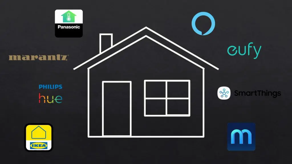
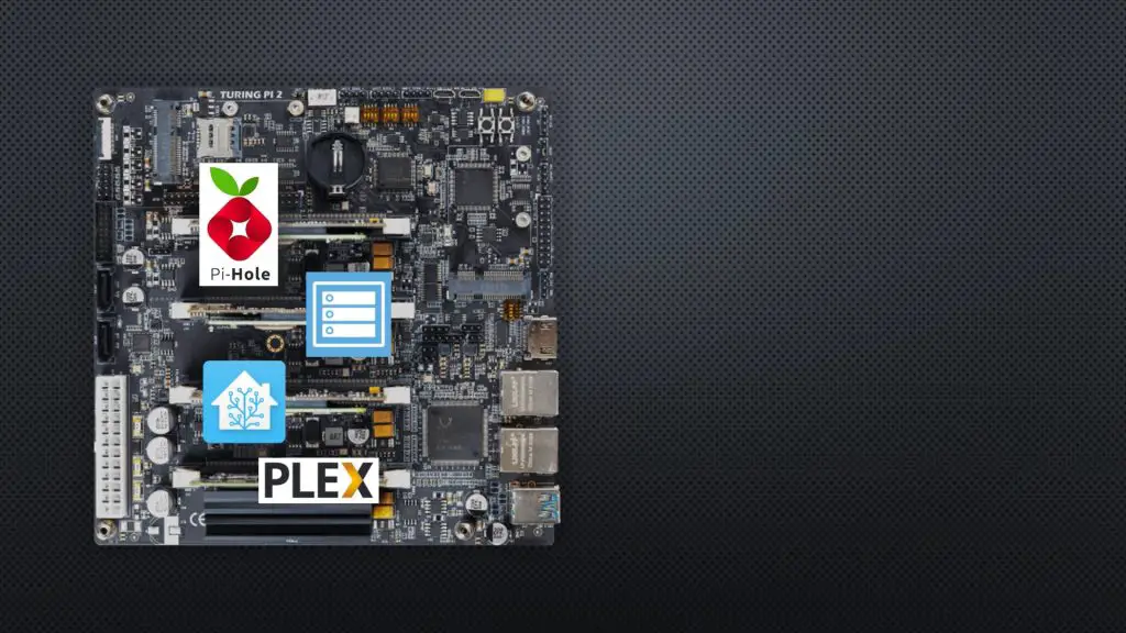
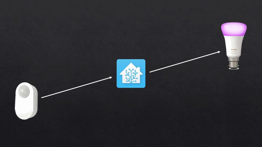
If you’ve done anything home automation related on a Raspberry Pi then you’ve probably heard of Home Assistant. It a free and open-source software package that is designed to be a central hub or control system for all of your smart home devices and it’s got a pretty substantial online community working on integration. So, for example, it allows you to do things you wouldn’t normally be able to do like use an Ikea motion sensor to turn on a Philips hue light. Something that isn’t supported by either ecosystem individually.
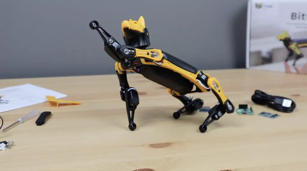
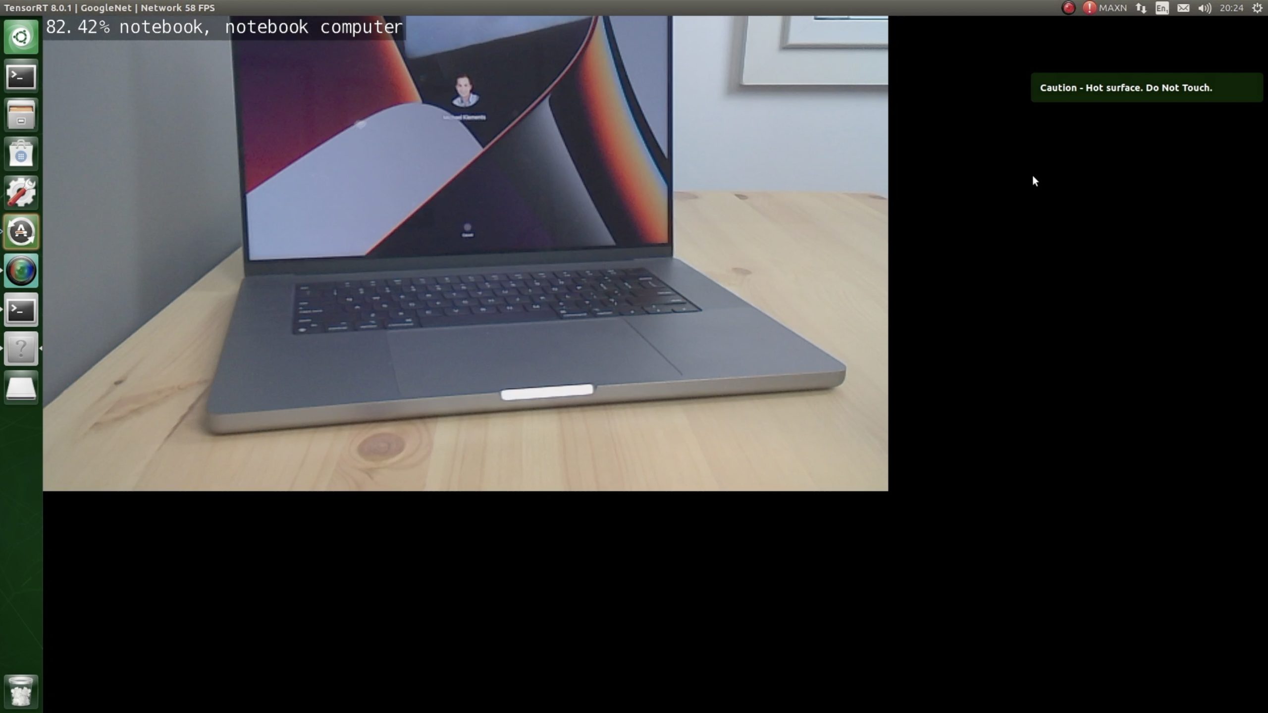
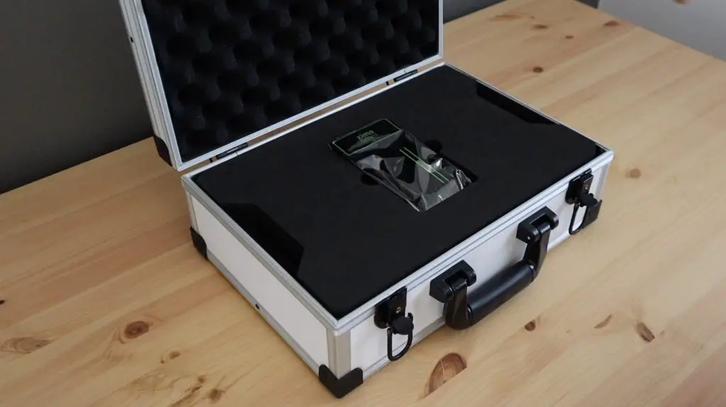
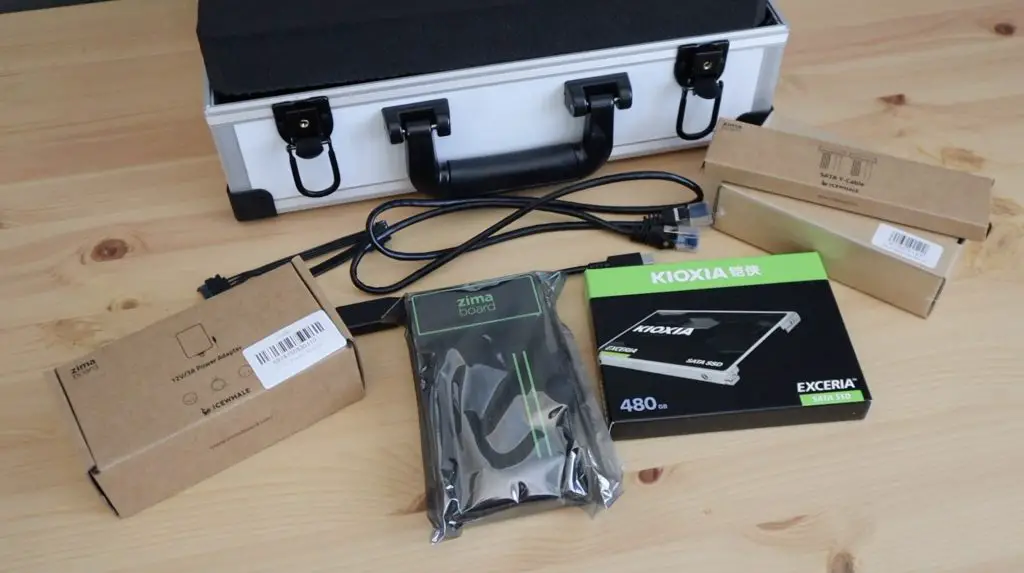
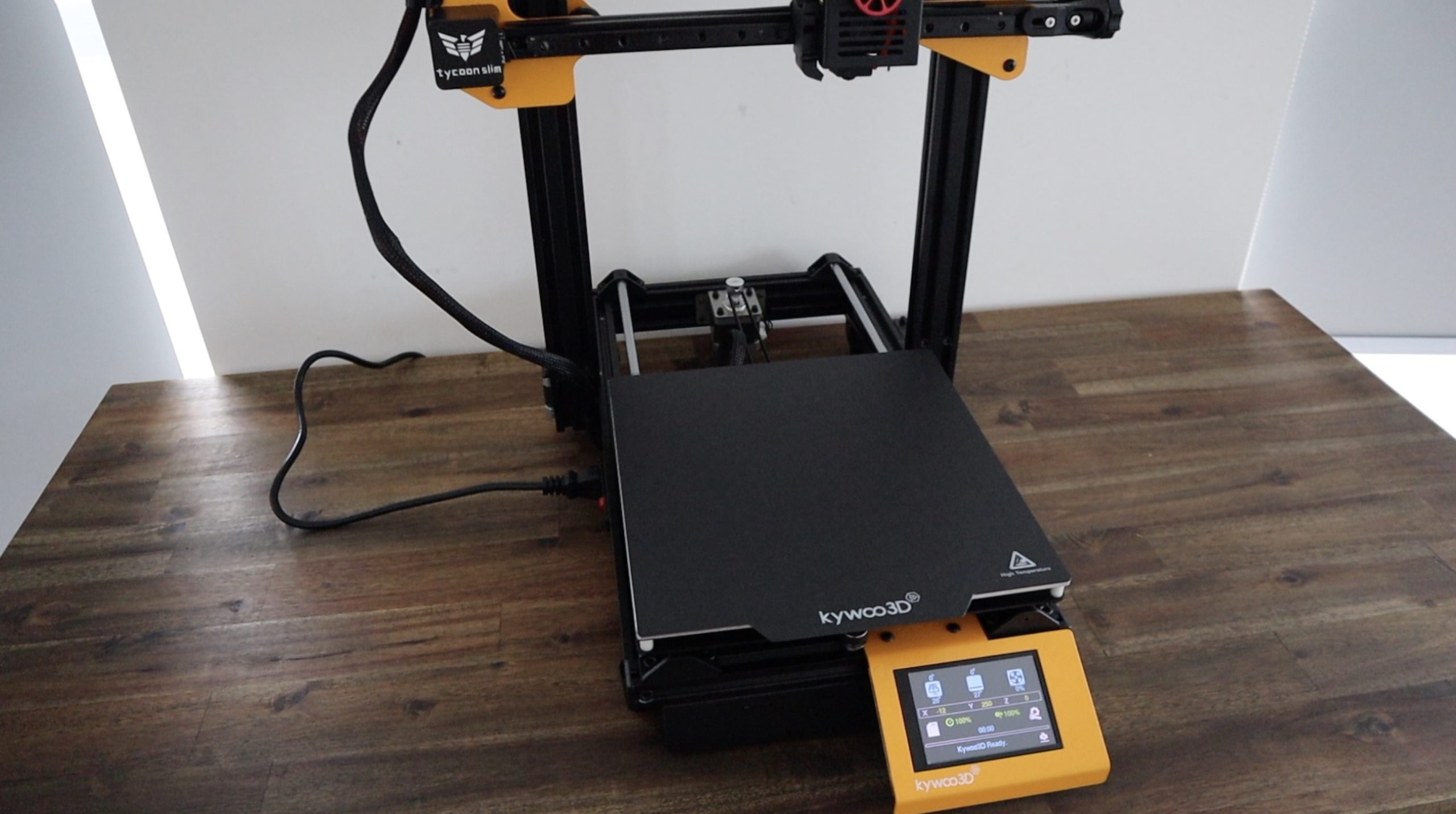
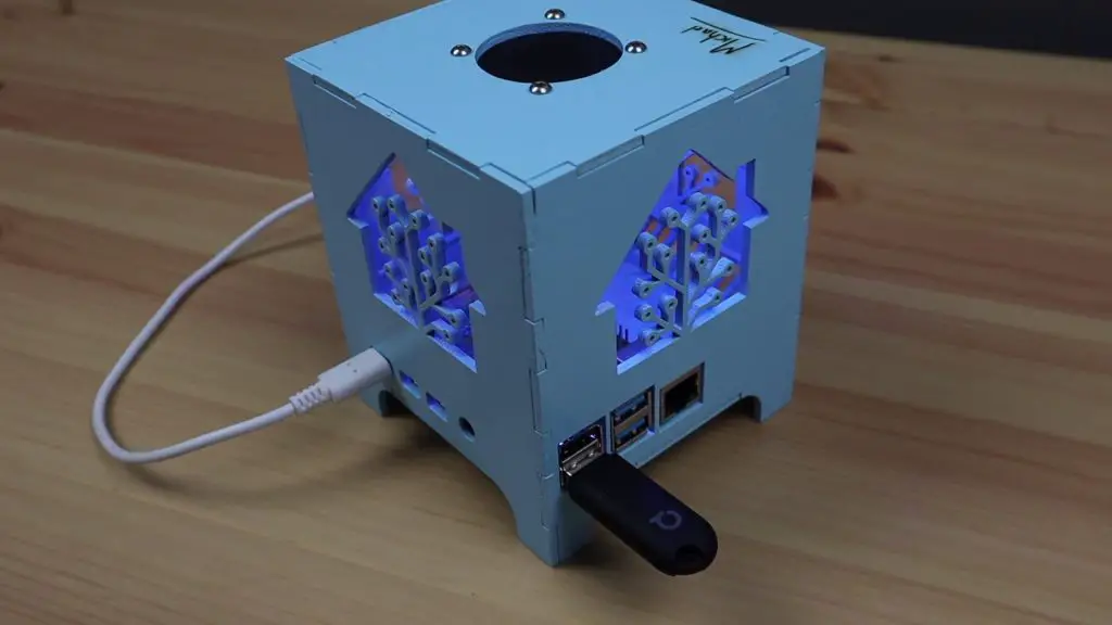
So today I’m going to be installing Home Assistant onto a Raspberry Pi and I’m going to use a new laser cutter, the Atomstack X20 Pro, to laser cut a housing for it so that I can put it somewhere convenient in my house without it looking like a jumble of wires, dongles and PCBs.
Here’s my video of the build, read on for the full write-up:
What You Need to Build Your Own Home Assistant Hub
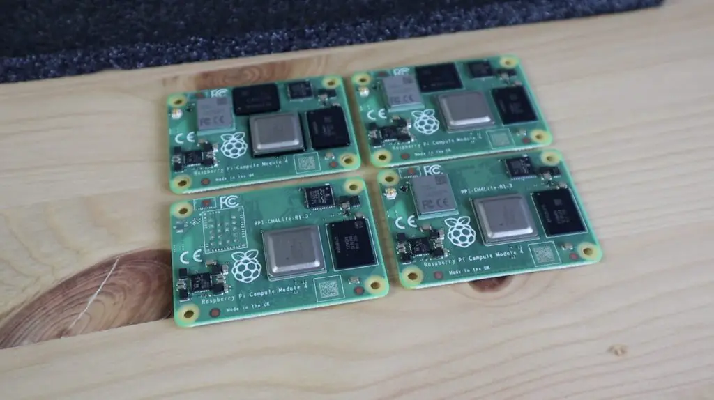
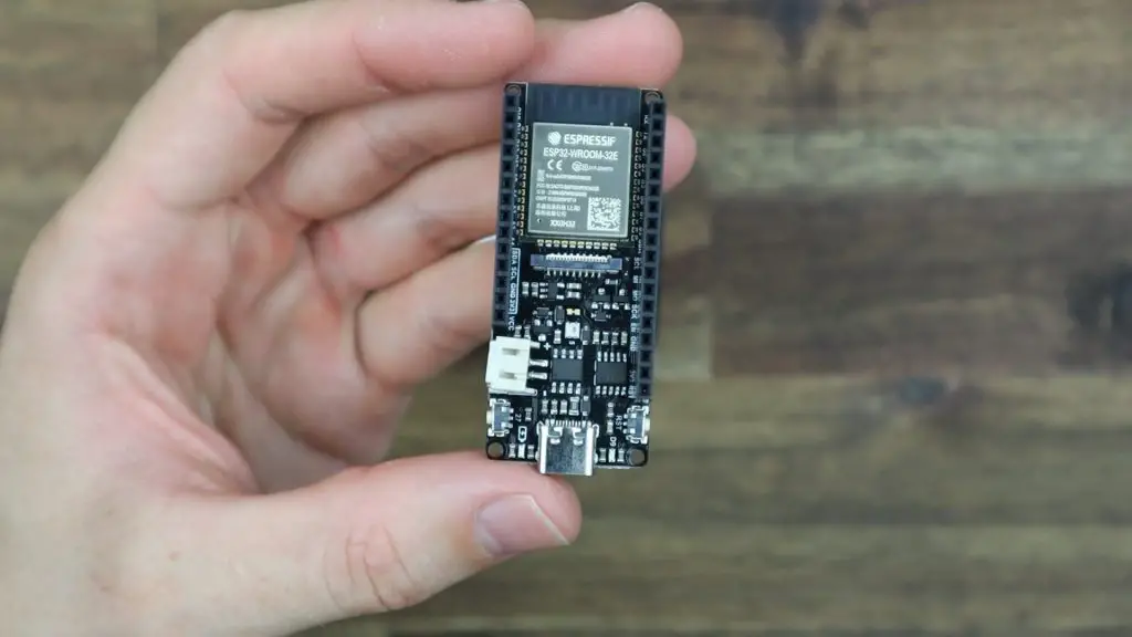
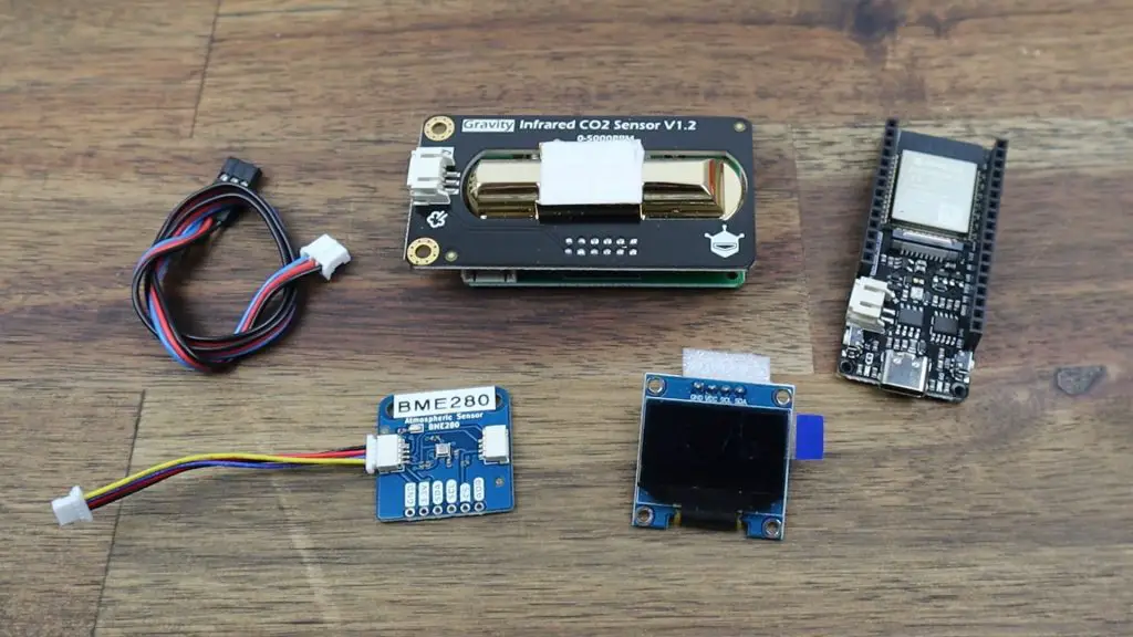
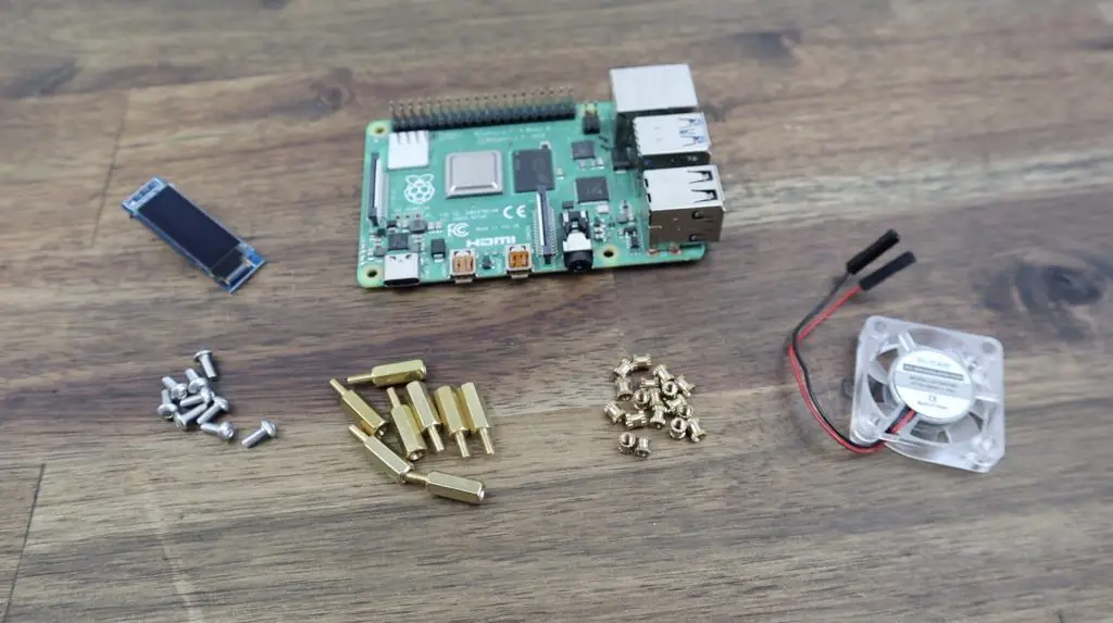
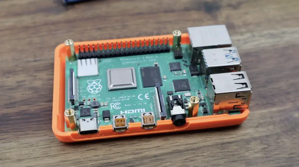
- Raspberry Pi 4B – Buy Here
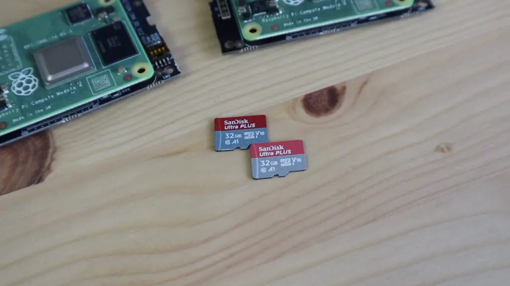
- 32GB Sandisk Ultra MicroSD Card – Buy Here
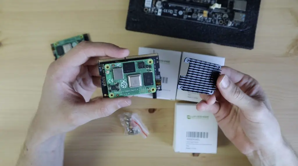
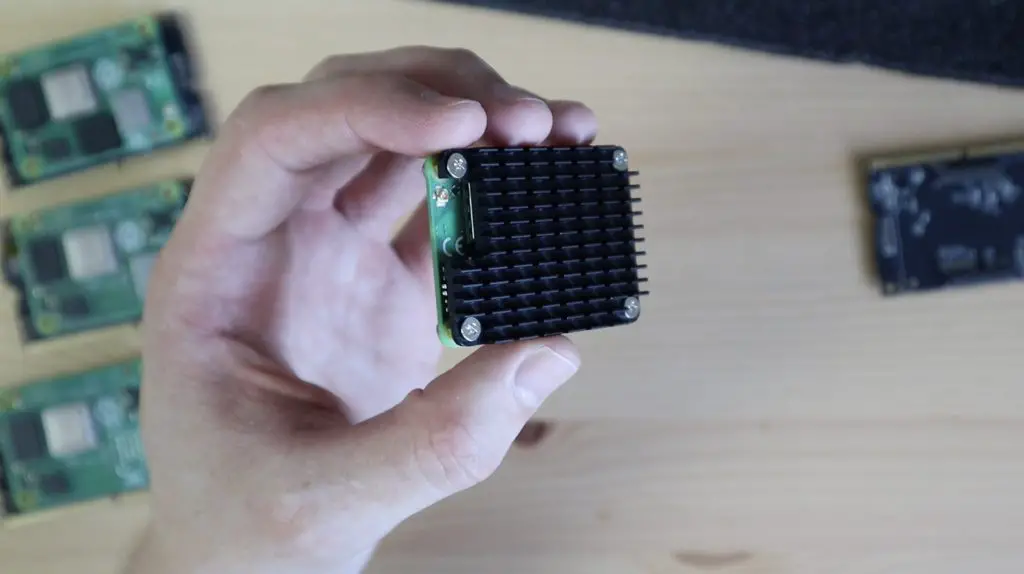
- Aluminium Heatsink – Buy Here
- Conbee II Zigbee Gateway – Buy Here
- M3x8mm Button Head Screws – Buy Here
- M3 Nuts – Buy Here
- M2.5 Brass Standoffs – Buy Here
- M2.5 Nuts – Buy Here
- M2.5 Screws – Buy Here
Equipment used:
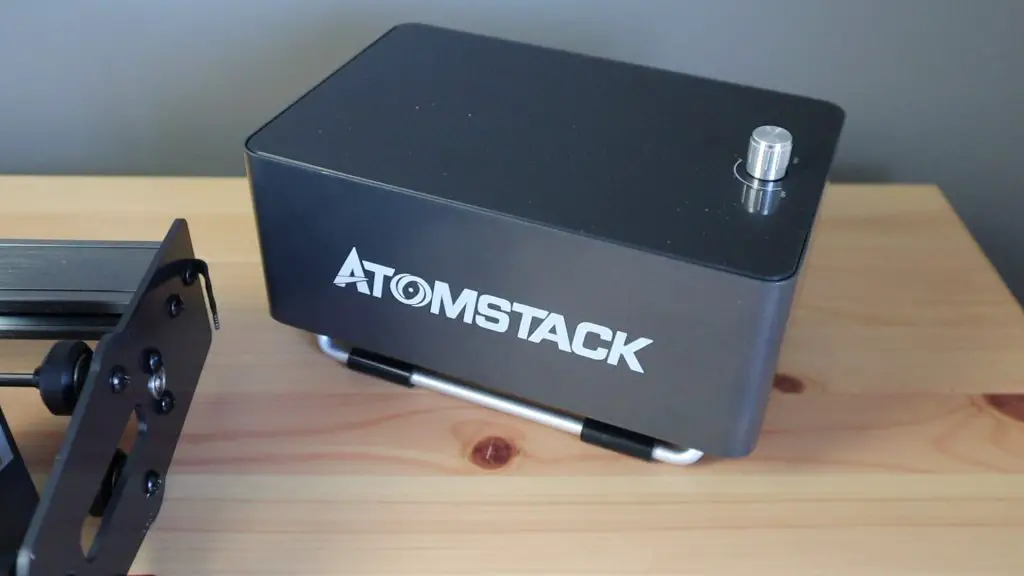
- Atomstack X20 Pro – Buy Here
- Electric Screwdriver – Buy Here
- Milwaukee Oscillating Multitool – Buy Here
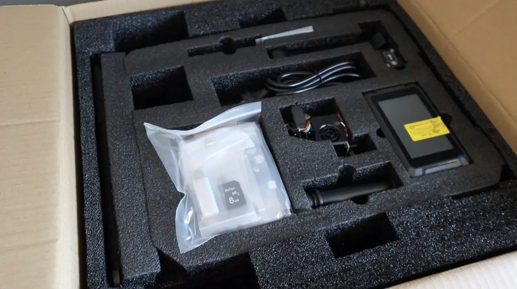
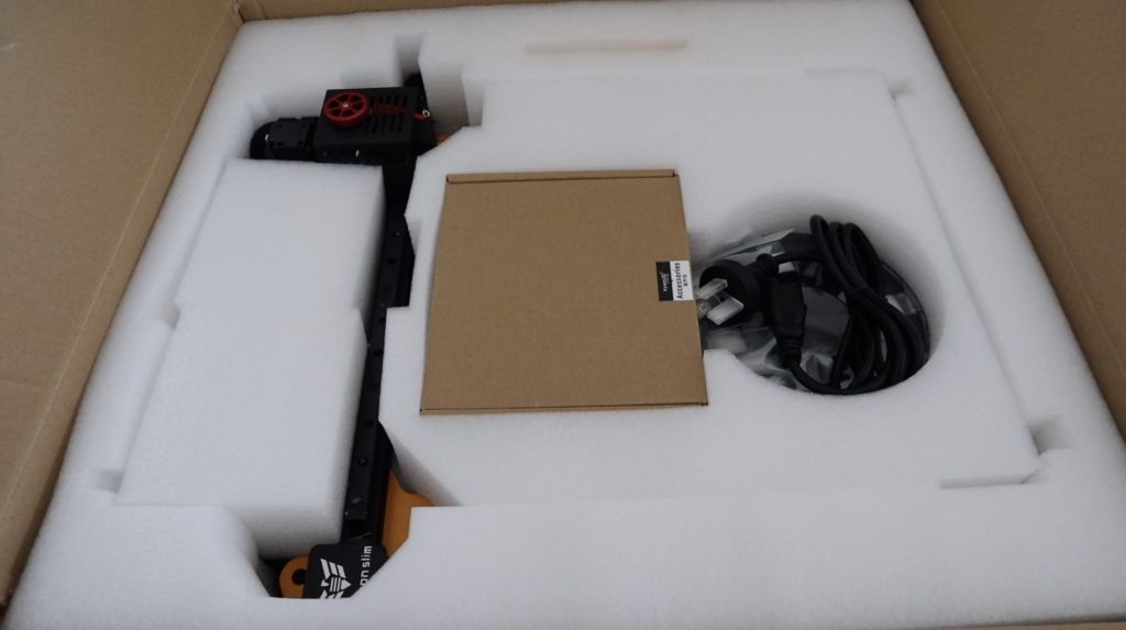
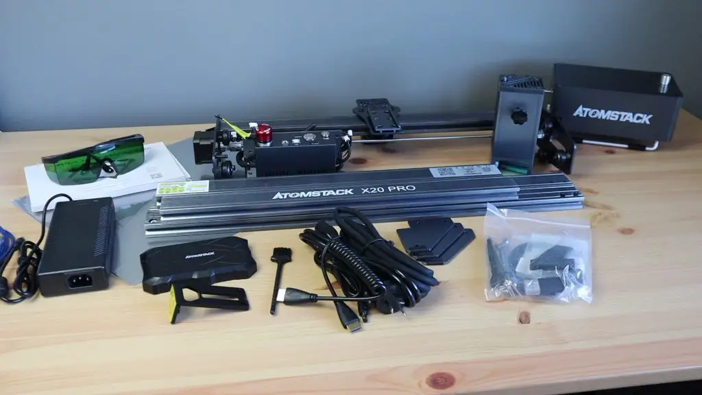
Unboxing and Setting Up The Atomstack X20 Pro
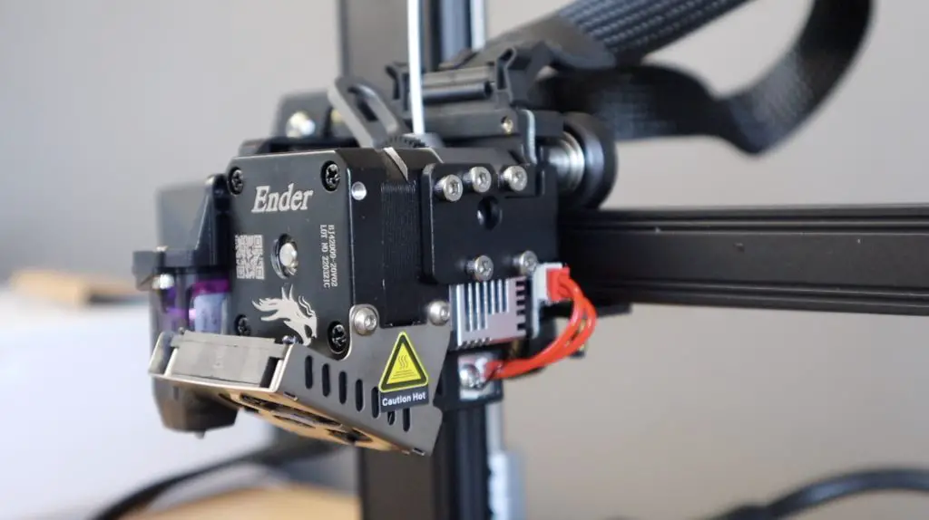
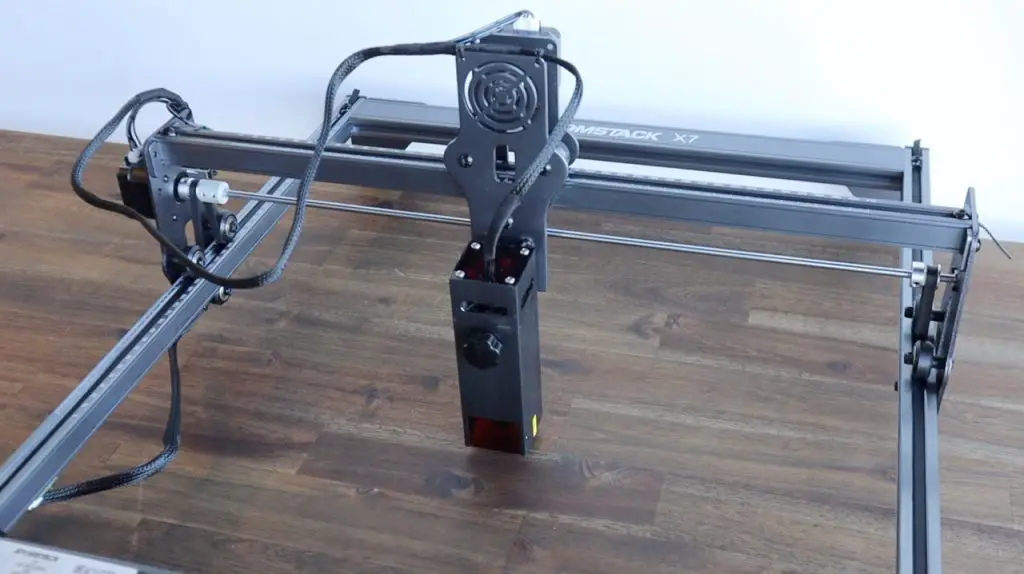
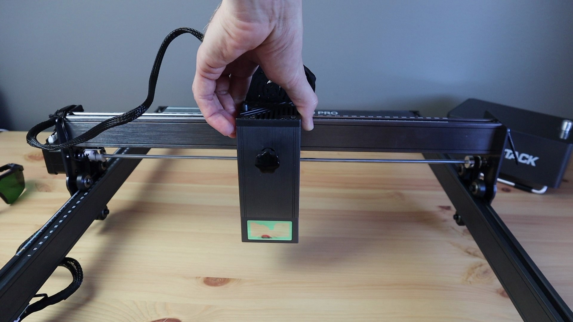
The X20 Pro is a new diode laser engraving and cutting machine from Atomstack that uses a clever quad diode laser module to deliver 20W of optical power. The laser is so powerful that they claim that it can even cut 0.05mm sheet metal, which as far as I can tell is a first for consumer-level diode lasers. They also say that I can cut up to 12mm sheets of wood in a single pass and up to 8mm sheets of opaque acrylic.
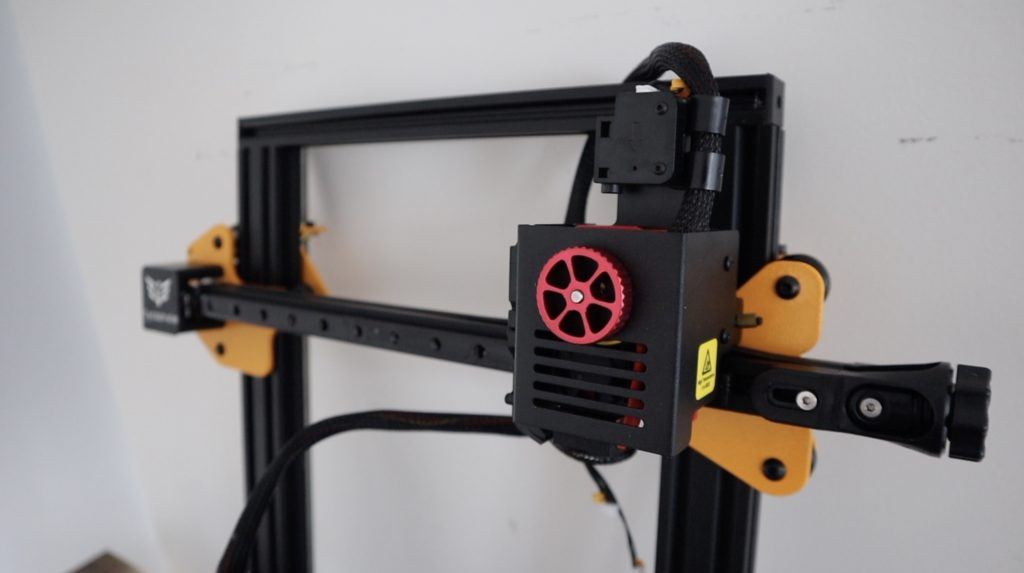
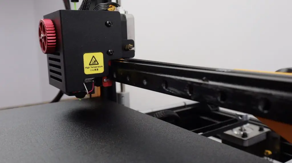
The 20W laser module is quite a bit stockier than the one on the X7.
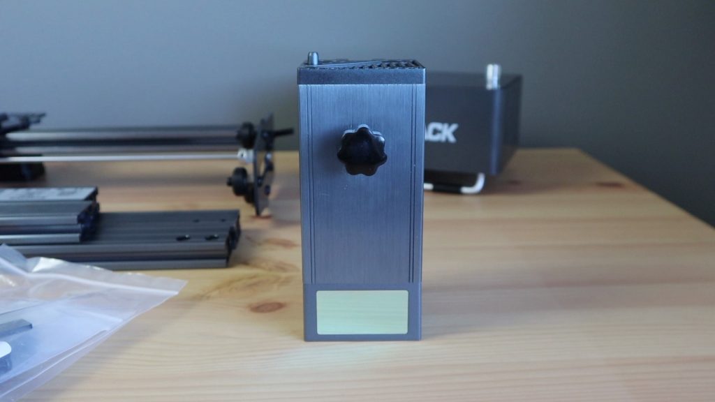
The control PCB and cooling fan are built into the metal housing and an air port on the top feeds down to a nozzle around the lens for the included air assist system. I really like how well the air assist system is integrated into the design of the module and doesn’t look like an afterthought.
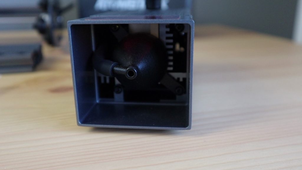
The included air assist is their own branded system. I’ve used an industrial aquarium air pump previously on my K40 laser cutter, so I was expecting this to be something along those lines, but it’s actually a lot better. The unit apparently uses a two-cylinder compressor to deliver 10-25L/min of air to improve cutting and and engraving quality and speed, we’ll see how it works in a bit.
At a little over $1,000, it has a hefty price tag, so I’m hoping that this machine can do some cutting that’s at least equivalent to most entry-level 40W CO2 lasers.
So let’s get it assembled.
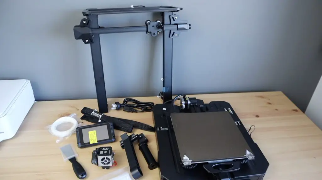
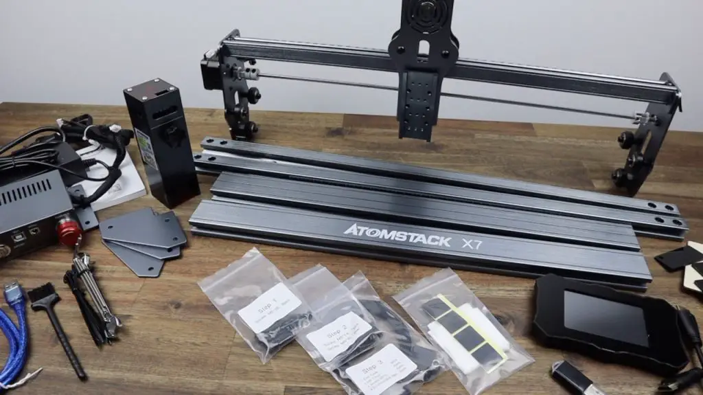
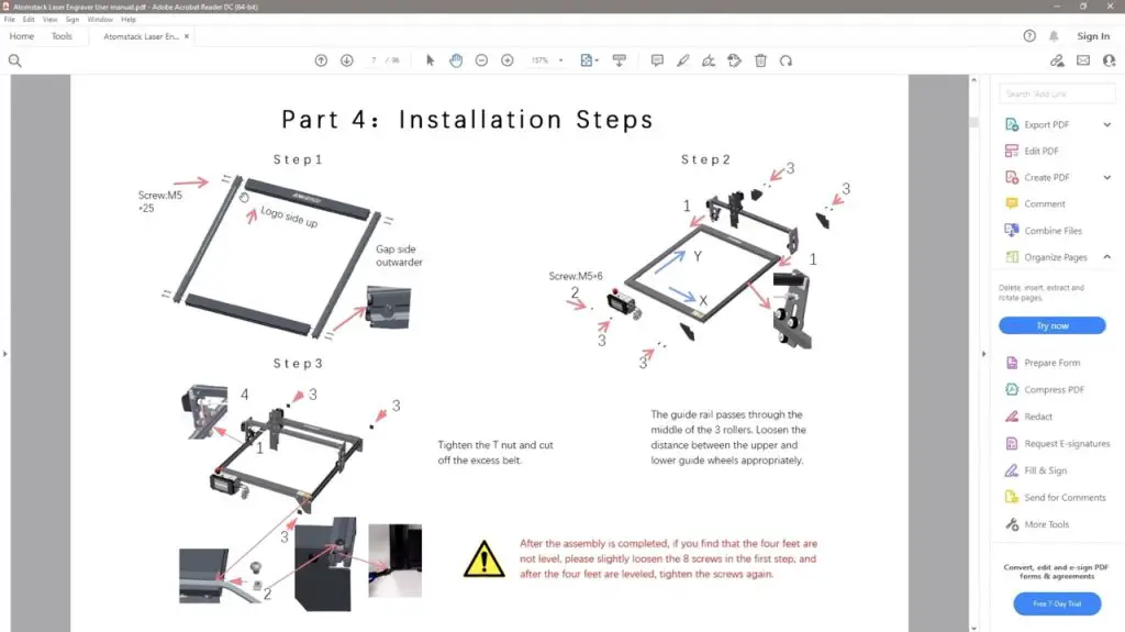
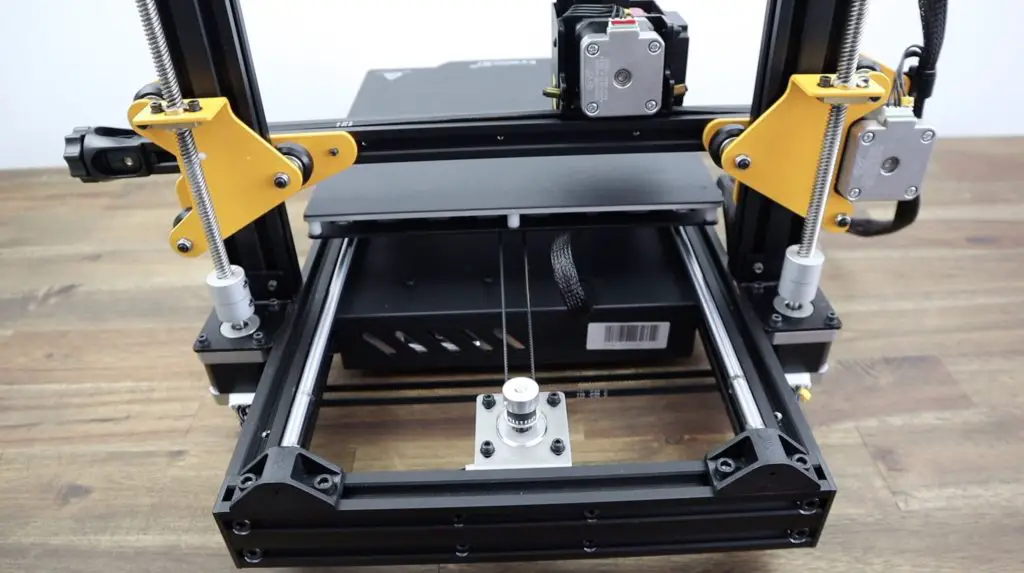
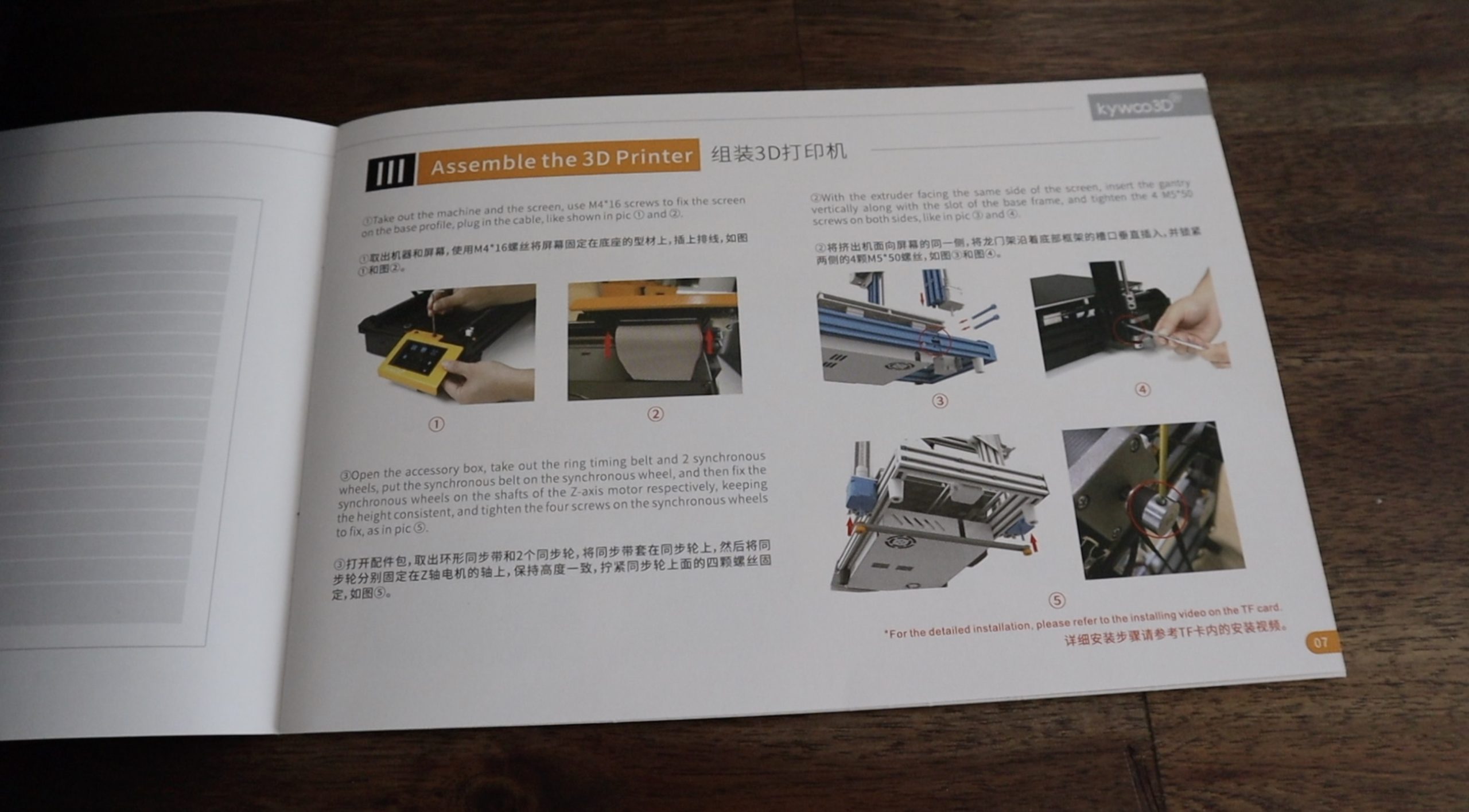
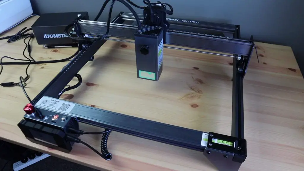
As with the X7 model, the X20 Pro comes largely preassembled, so assembly is pretty straight forward.
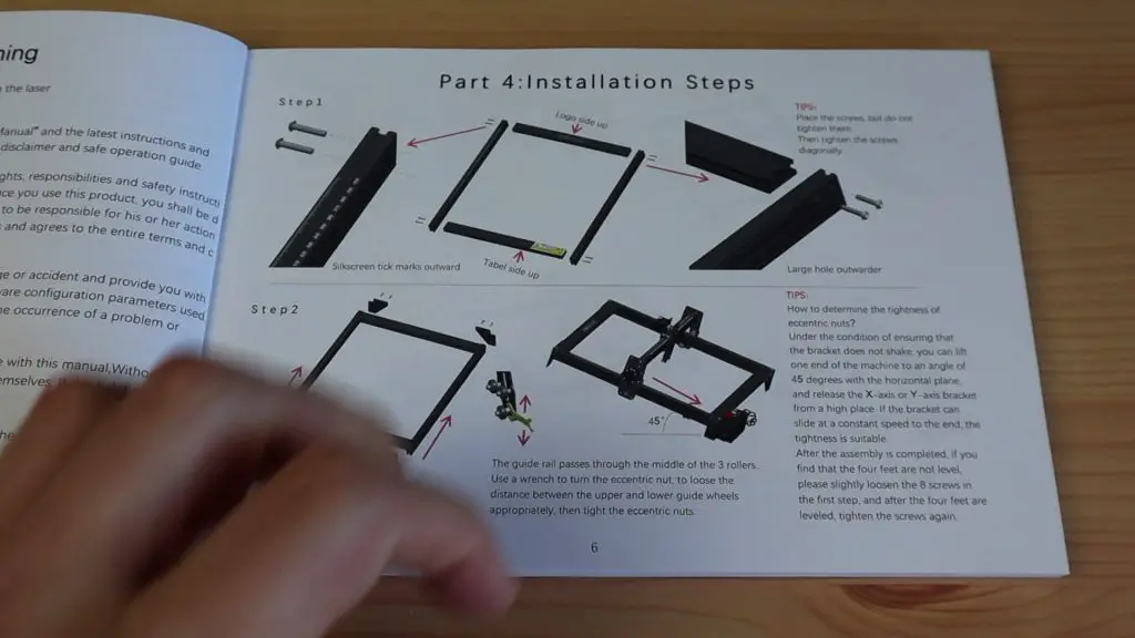
There are a couple of pages for assembly in the manual and the components are labelled for each step, so they’ve made it really easy.
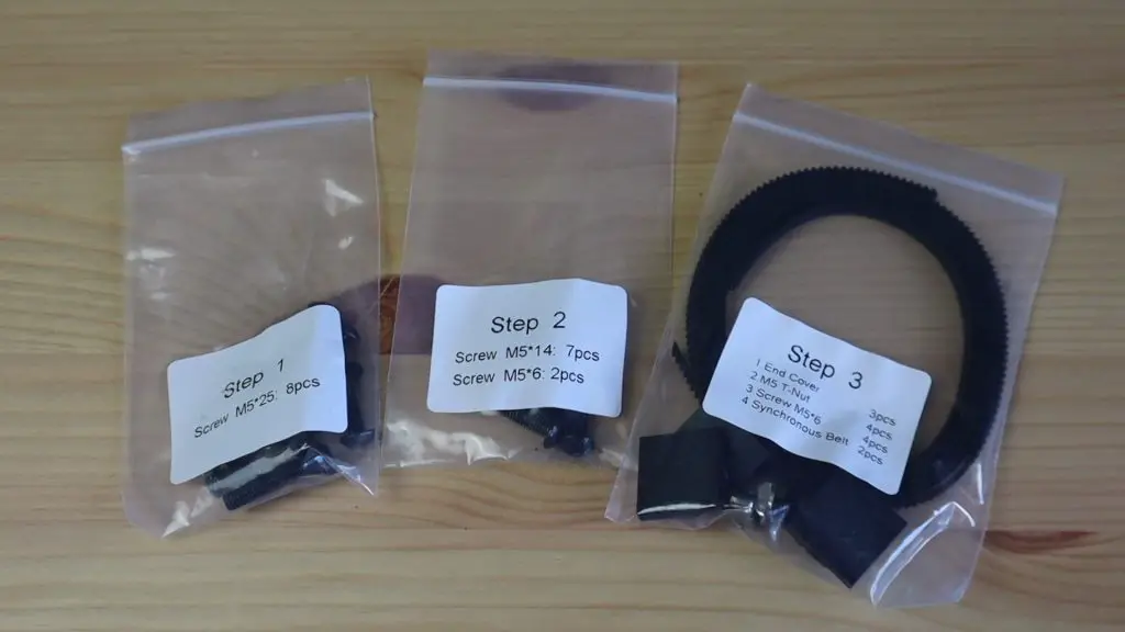
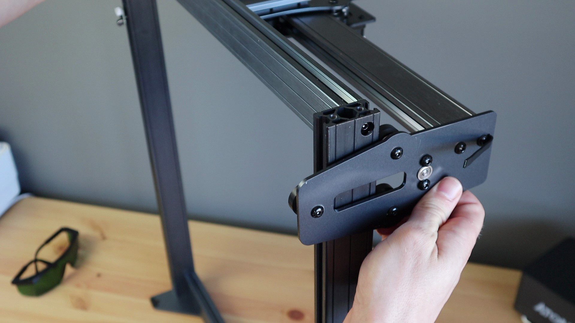
The gantry is all pre-assembled so you mainly need to assemble the four-sided frame and then mount the gantry and belts onto it along with the laser module. The only fiddly job is feeding the belts through the gantry wheels and toothed pulley on either side.
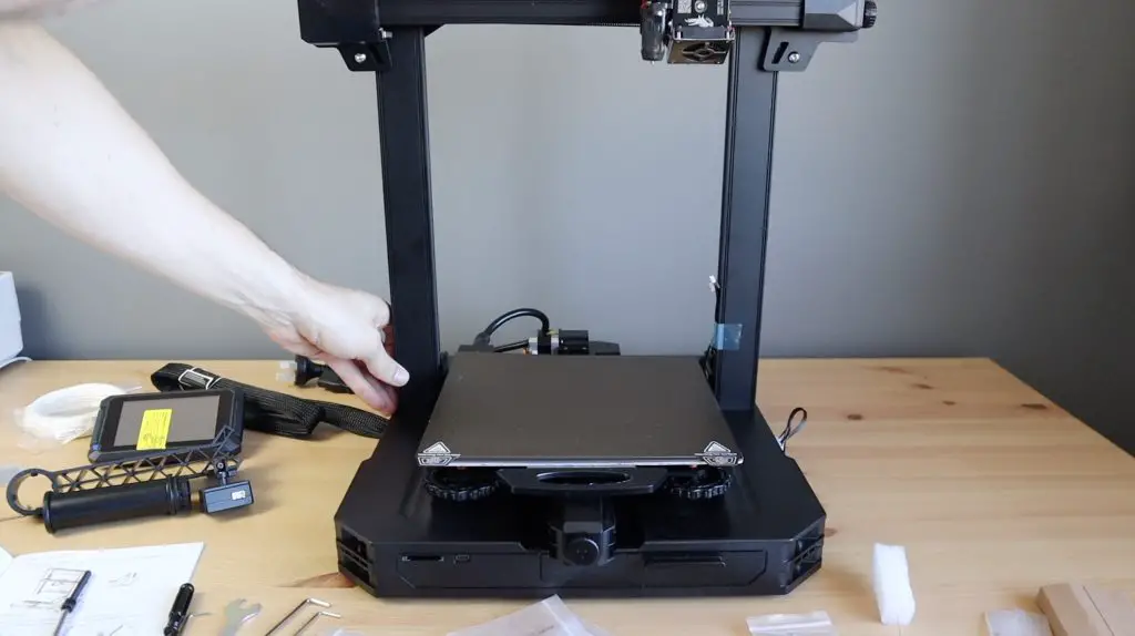
It took me about 20 minutes to assemble the X20 Pro and to adjust the legs so that it sat perfectly flat on my desk.
Test Cut and Engraving on The X20 Pro
I then tried turning it on, particularly to try the air assist pump to see how loud it would be. I have to say that I was pleasantly surprised. The industrial aquarium pump that I’ve used in the past is basically as loud as a standard workshop compressor. This system is substantially quieter in comparison.
It makes quite a noise if you turn the power all the way up, but you probably don’t need to use it at more than half power for most applications. You can feel a decent amount of air coming out of the nozzle at half speed, and you’ll then hardly hear it over the fan on the actual laser module (which is quite loud for a laser module). Even at full speed its quiet enough to comfortably talk over and you don’t feel like you need hearing protection when its running. It’s not something that you’re going to want to leave running unnecessarily but it’s definitely bearable for a small workshop.
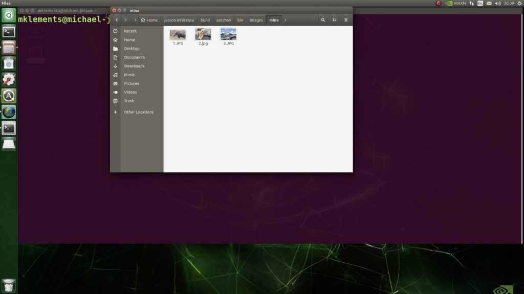
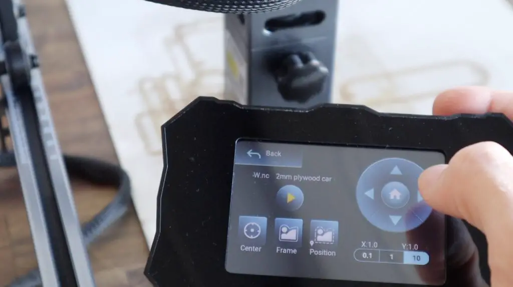
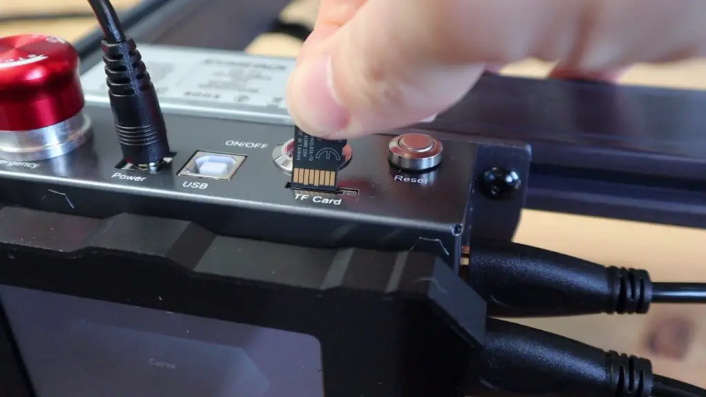
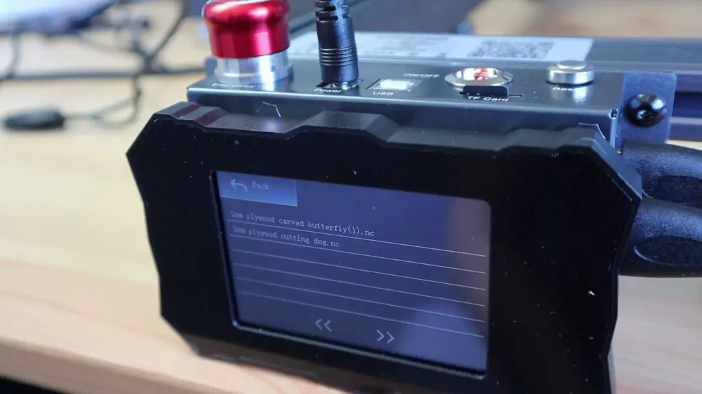
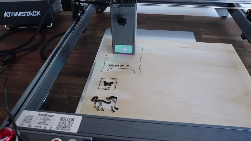
If we plug in the included MicroSD card, there are two test files ready to go, one to cut and one to engrave.
So let’s try those out first, I’m going to get it moved to my workshop so I don’t burn a hole in my desk.
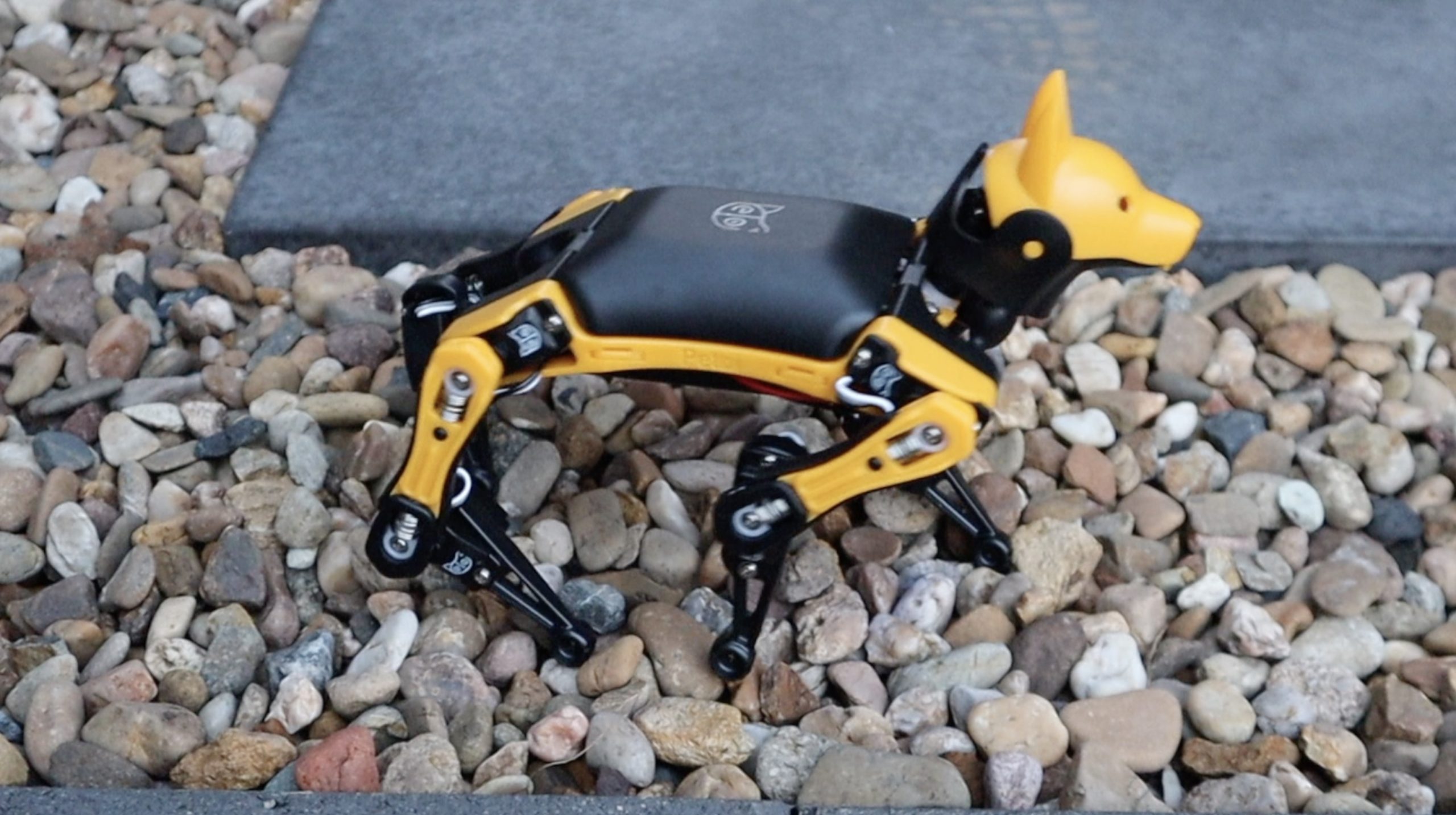
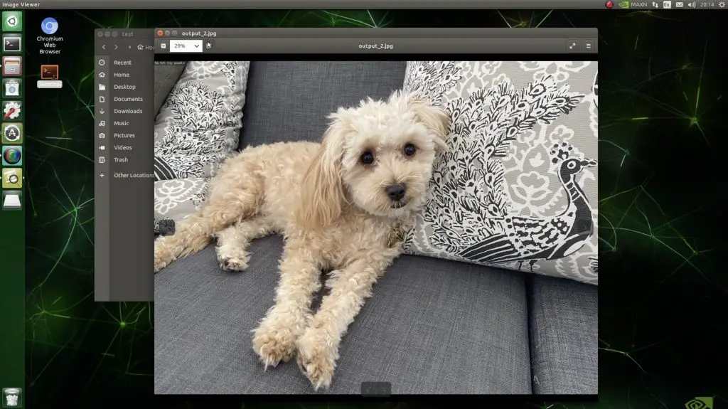
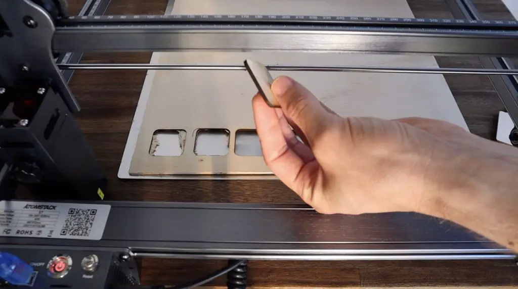
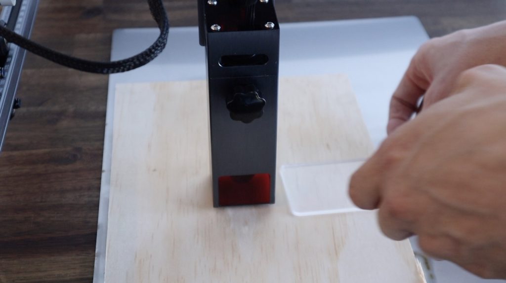
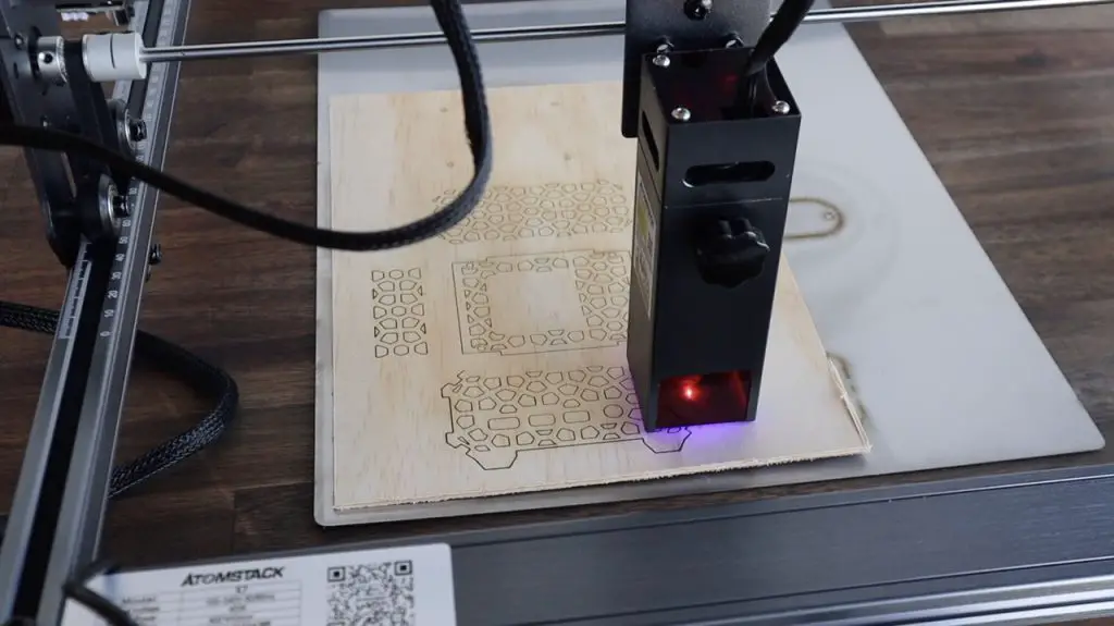
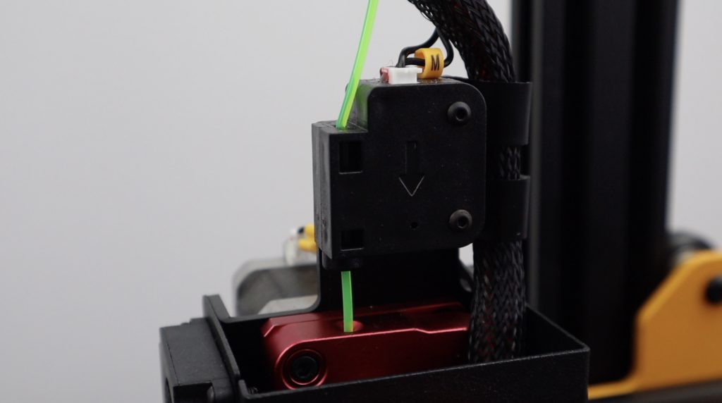
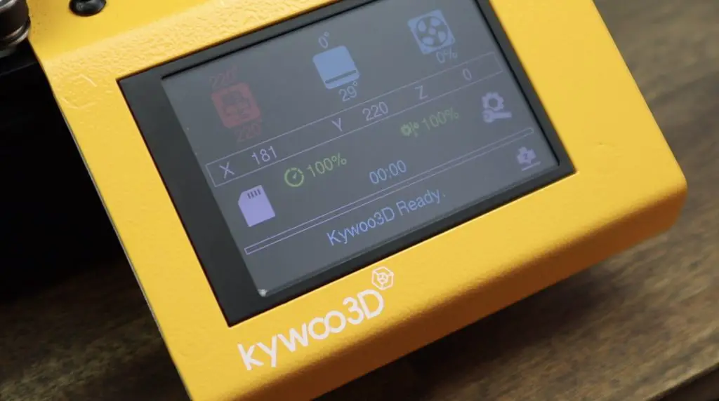
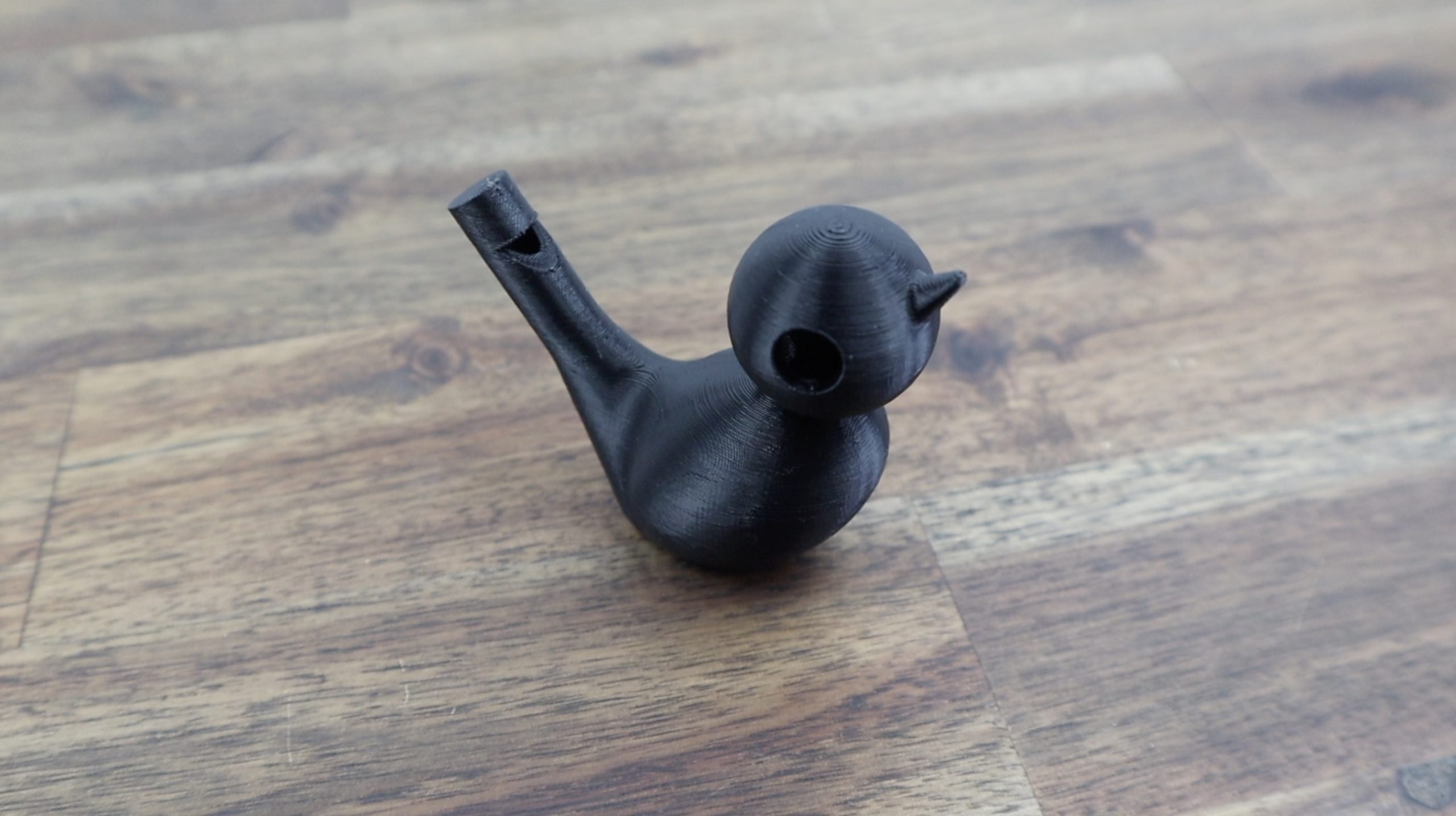
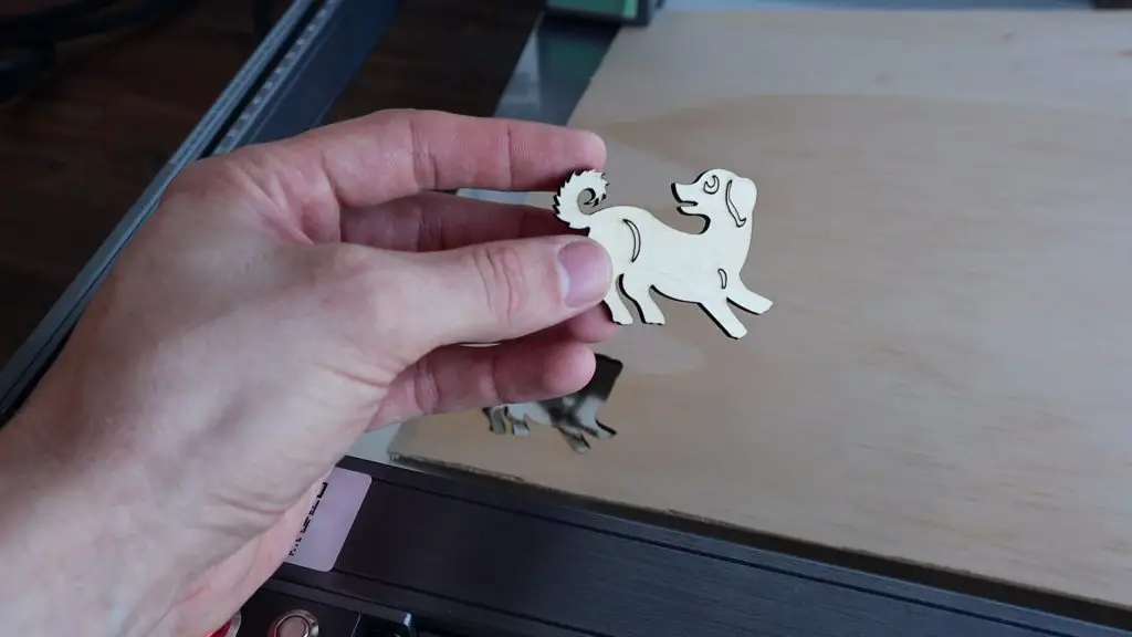
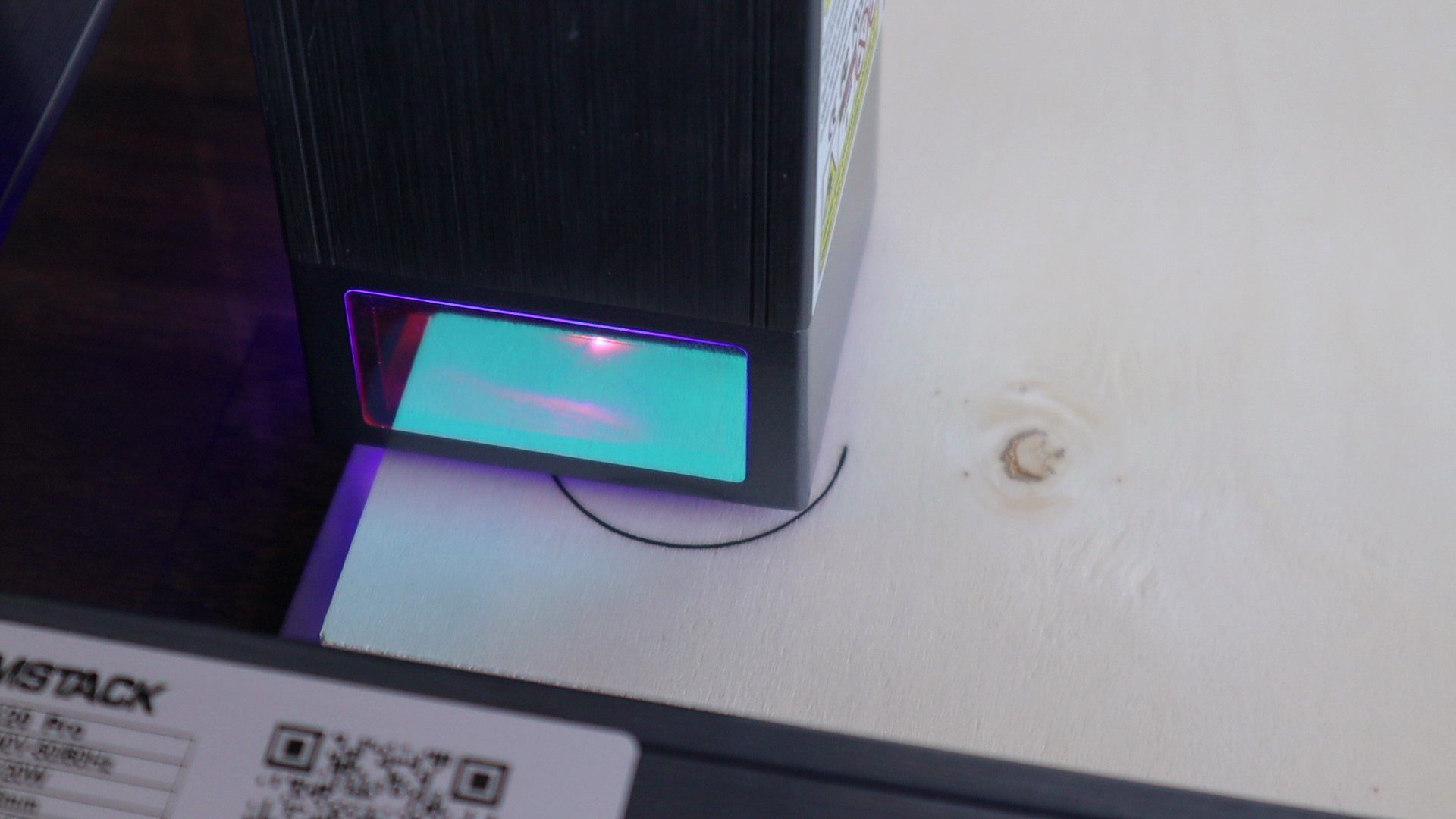
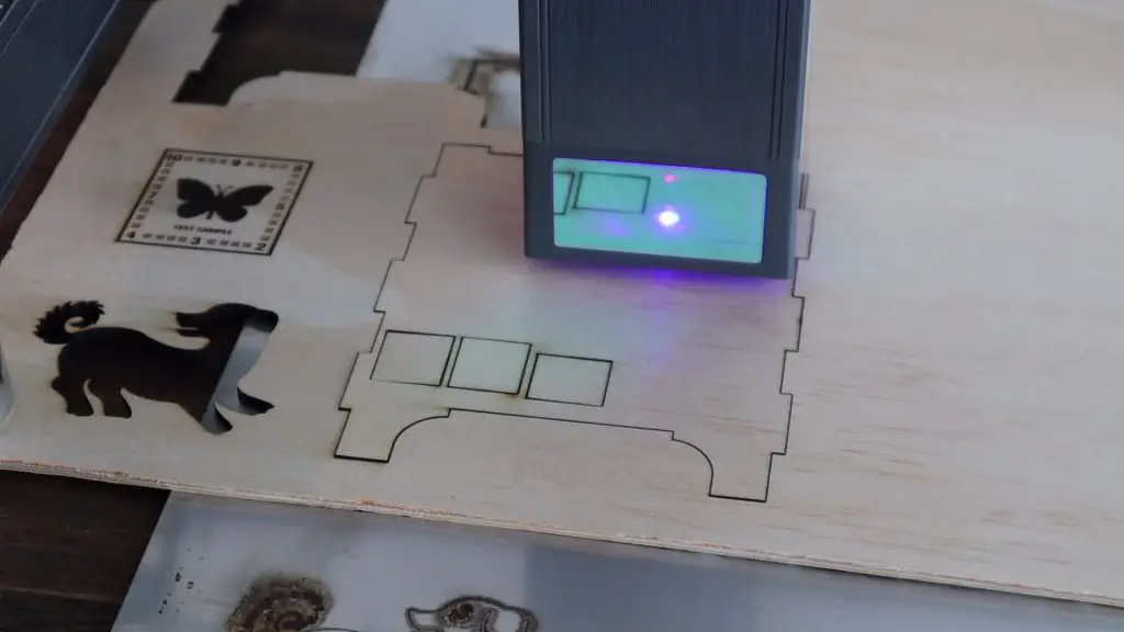
The first file is a dog that was labelled to be used on 2mm plywood. I’ve only got 3mm plywood so I thought I might need to do a second pass to cut all the way through. I used the offline controller to position the laser and run the test cutting file and I used the included distance tool to set the focus distance between the laser and the wood.
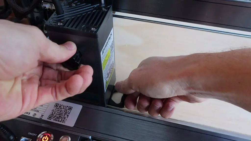
The laser seemed to cope just fine with the 3mm plywood and made quick work of the dog, cutting through the sheet in a single pass.
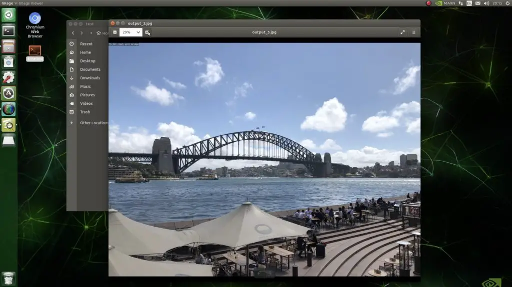
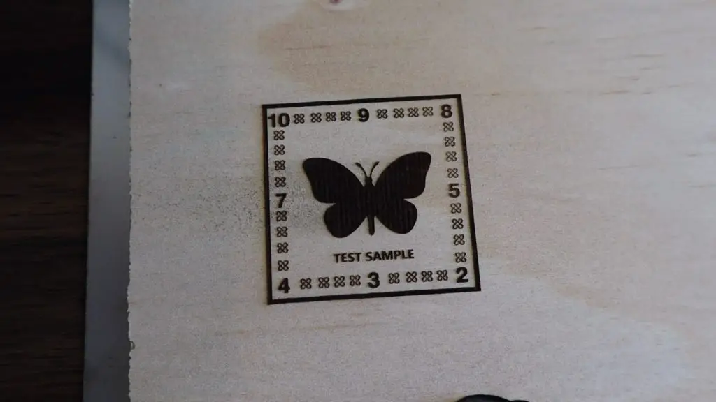
I then tried the engraving and that too produced a great quality finish with the air assist on about 30% power. There is some debate as to whether air assist is required when engraving as it tends to blow the smoke back onto the piece. I still prefer using some masking tape over the wood that I peel off after engraving – this produces flawless results every time.
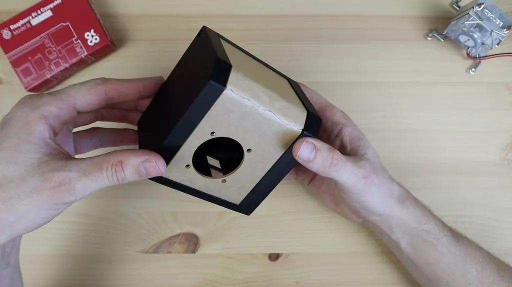
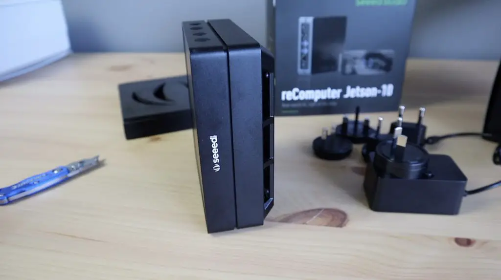
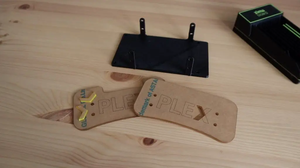
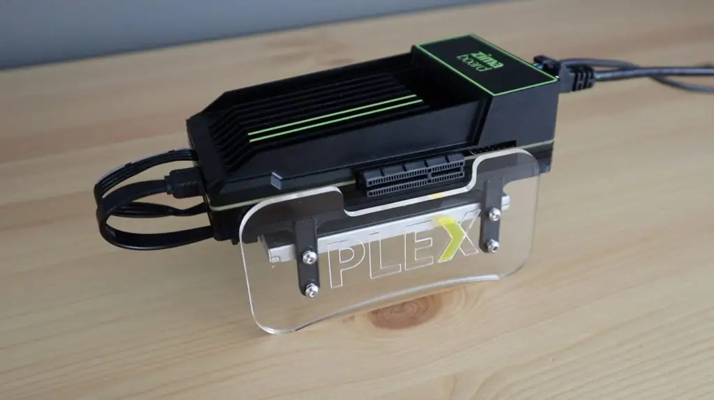
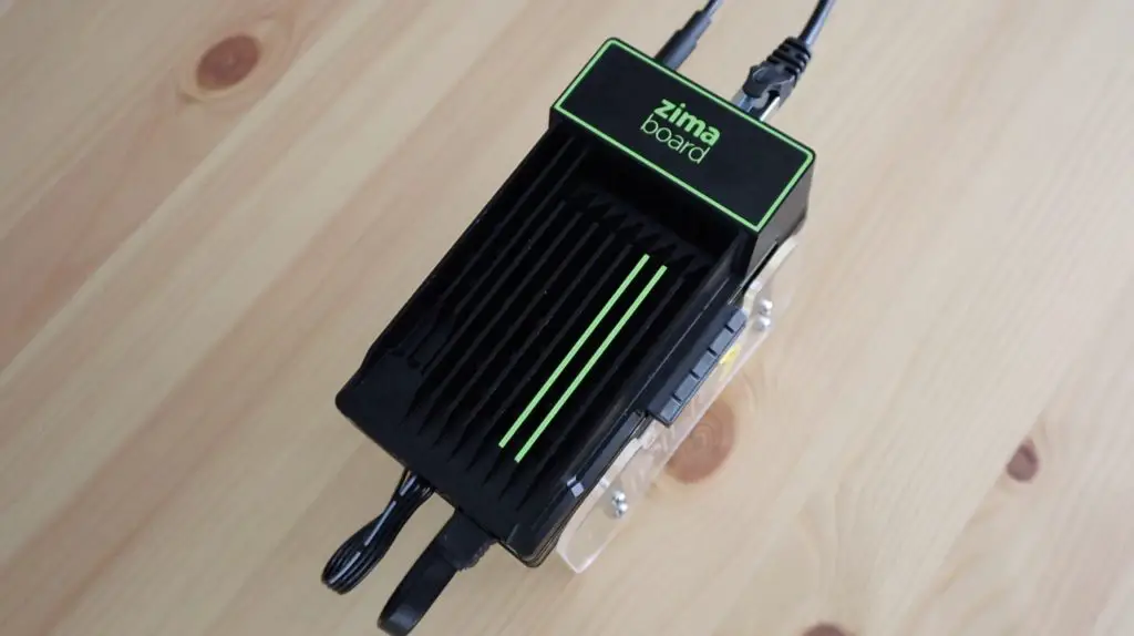
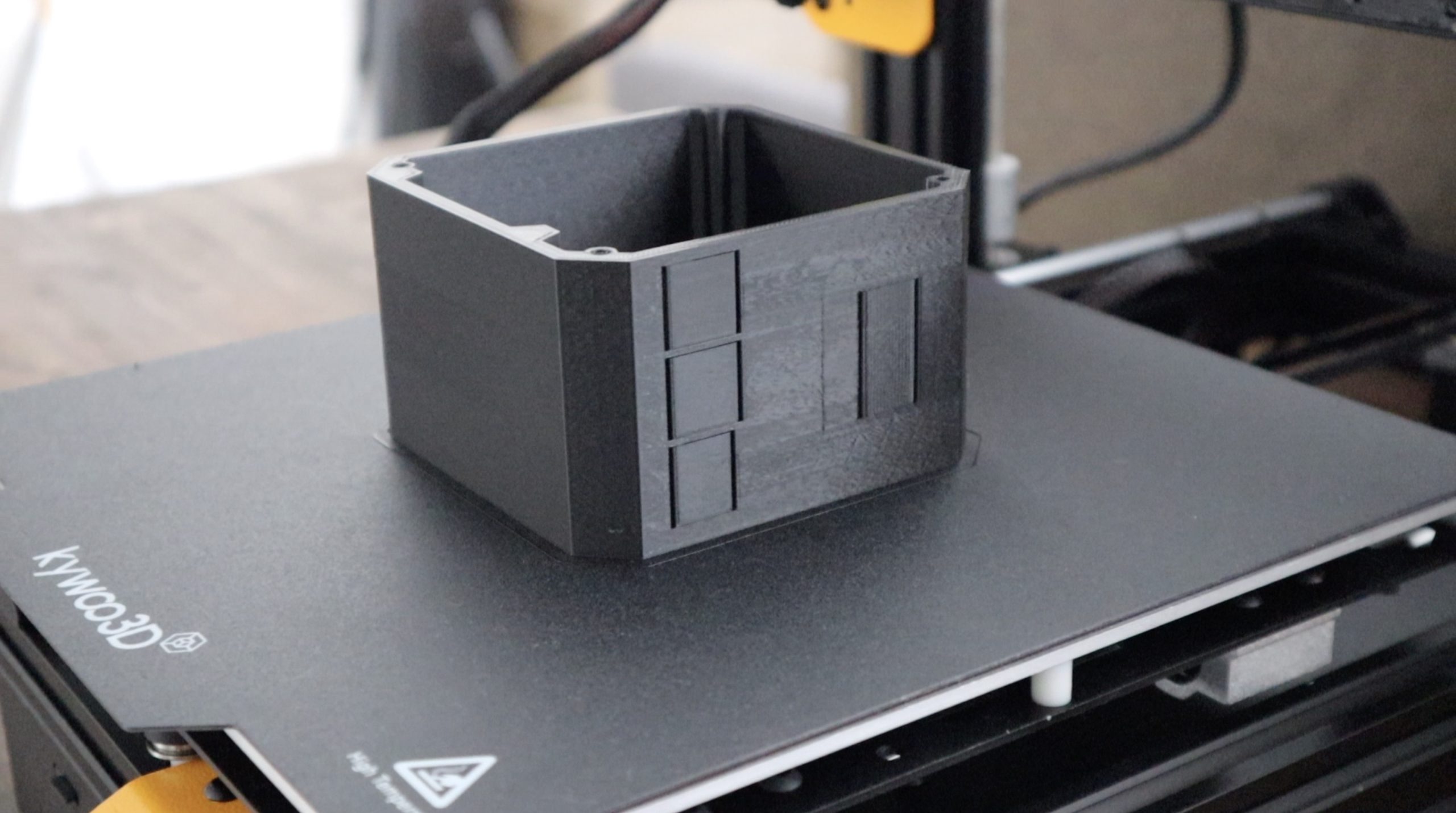
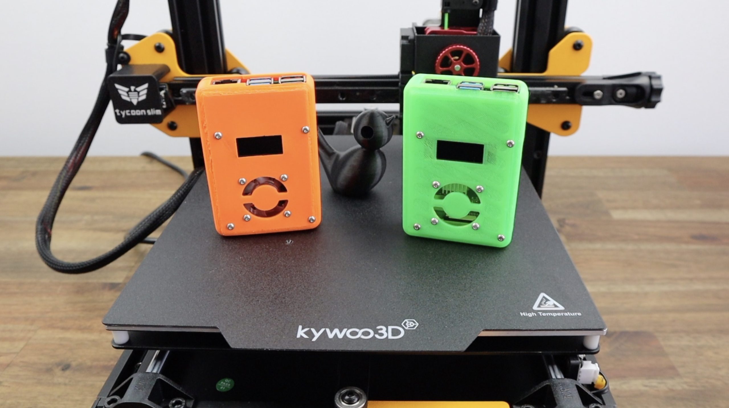
It looks like the X20 Pro is ready to take on a project, so we need to design the housing to hold the Raspberry Pi.
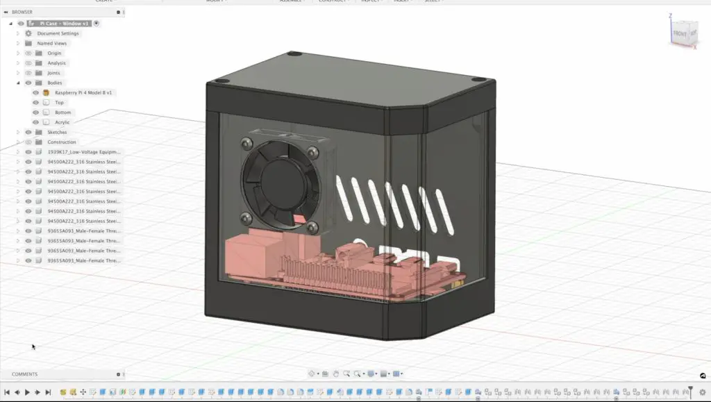
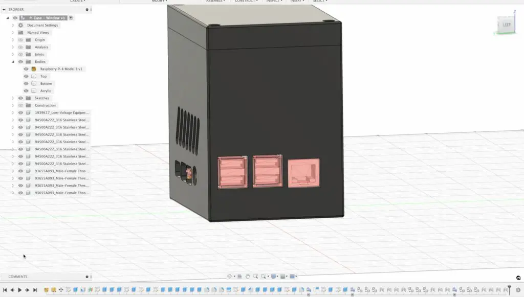
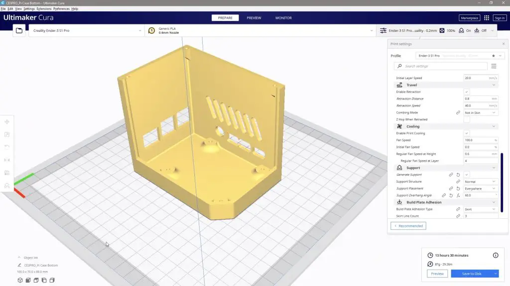
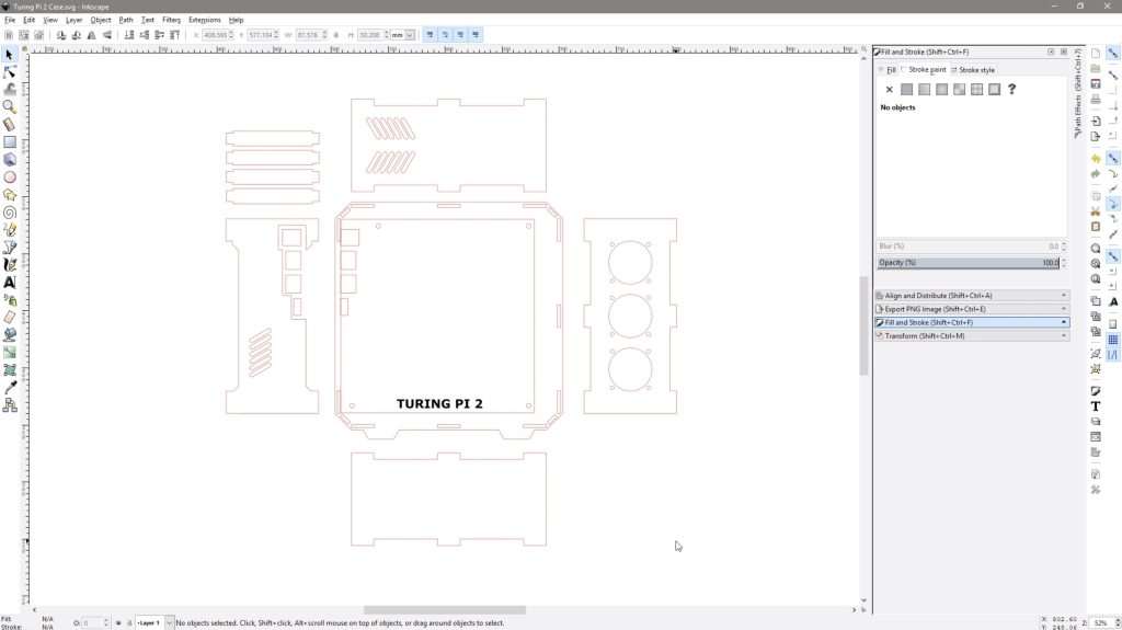
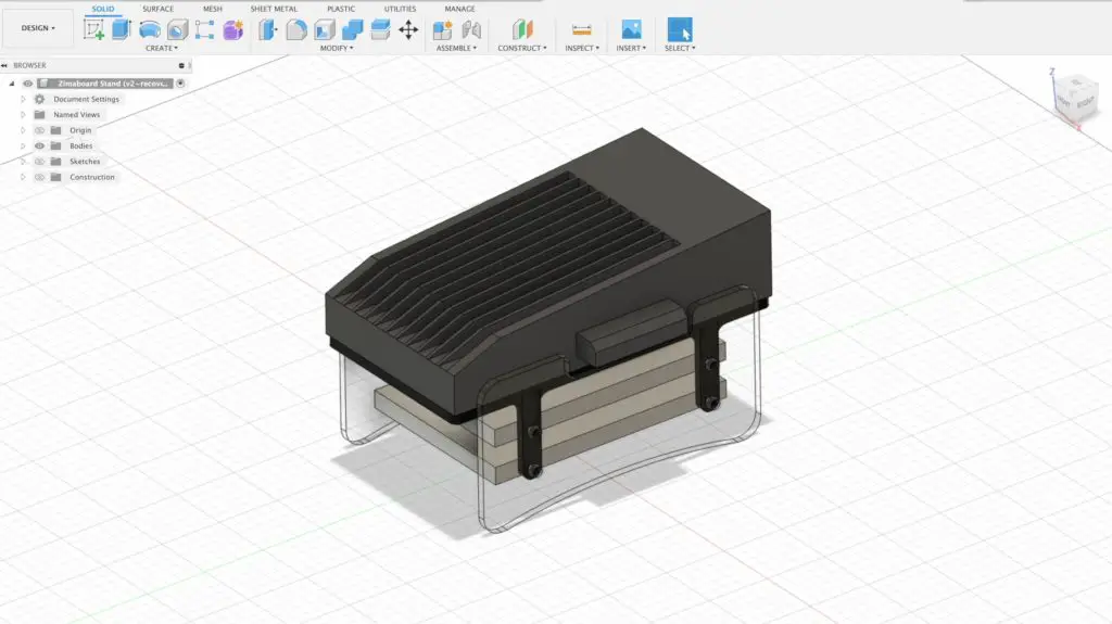
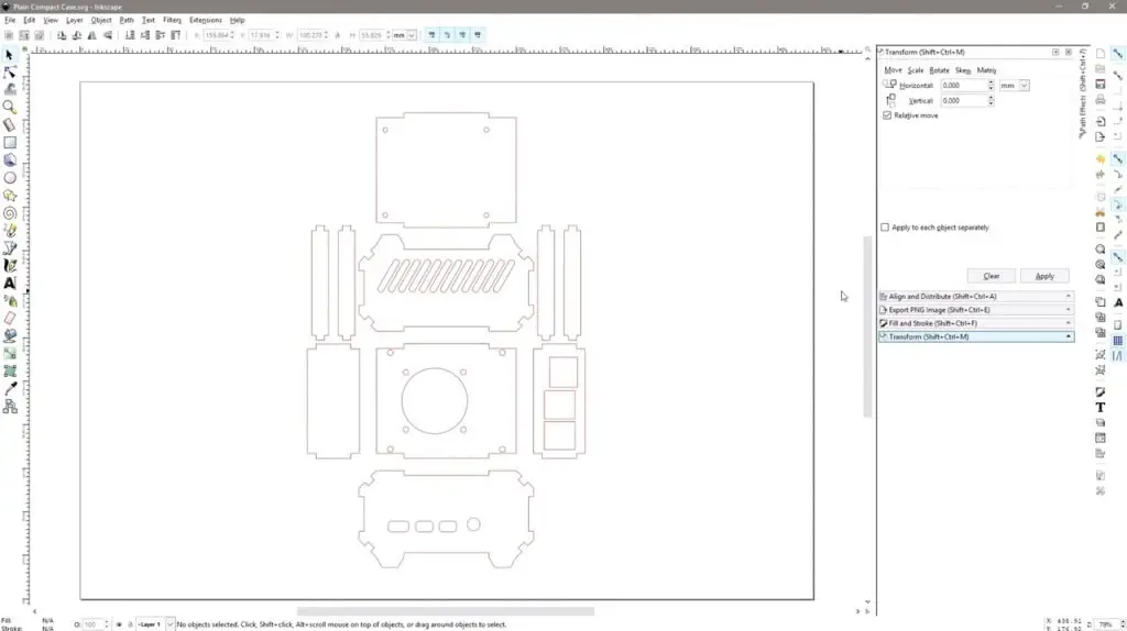
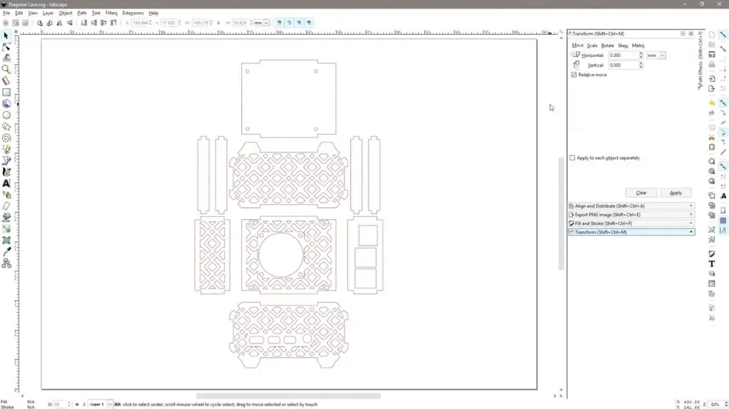
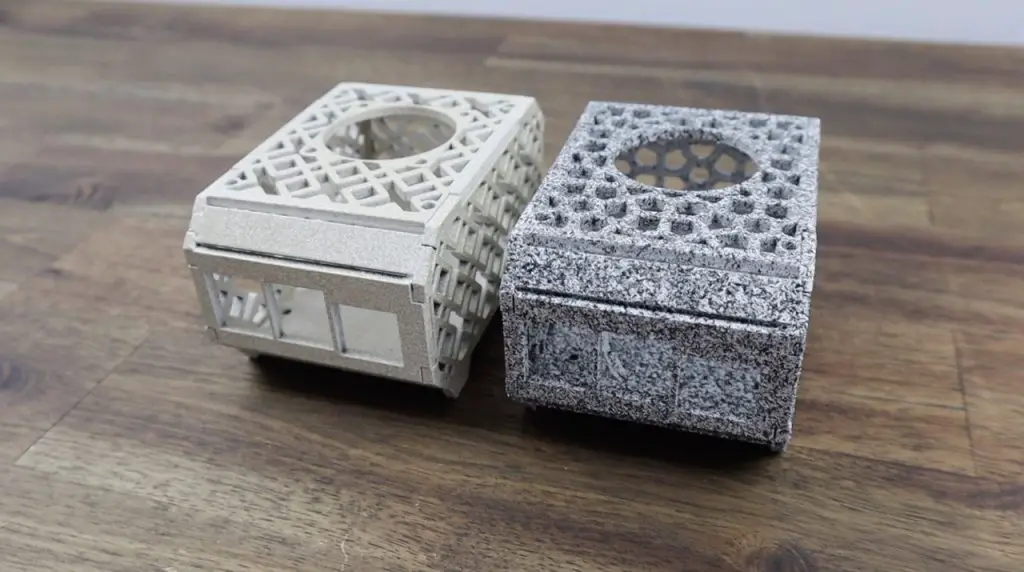
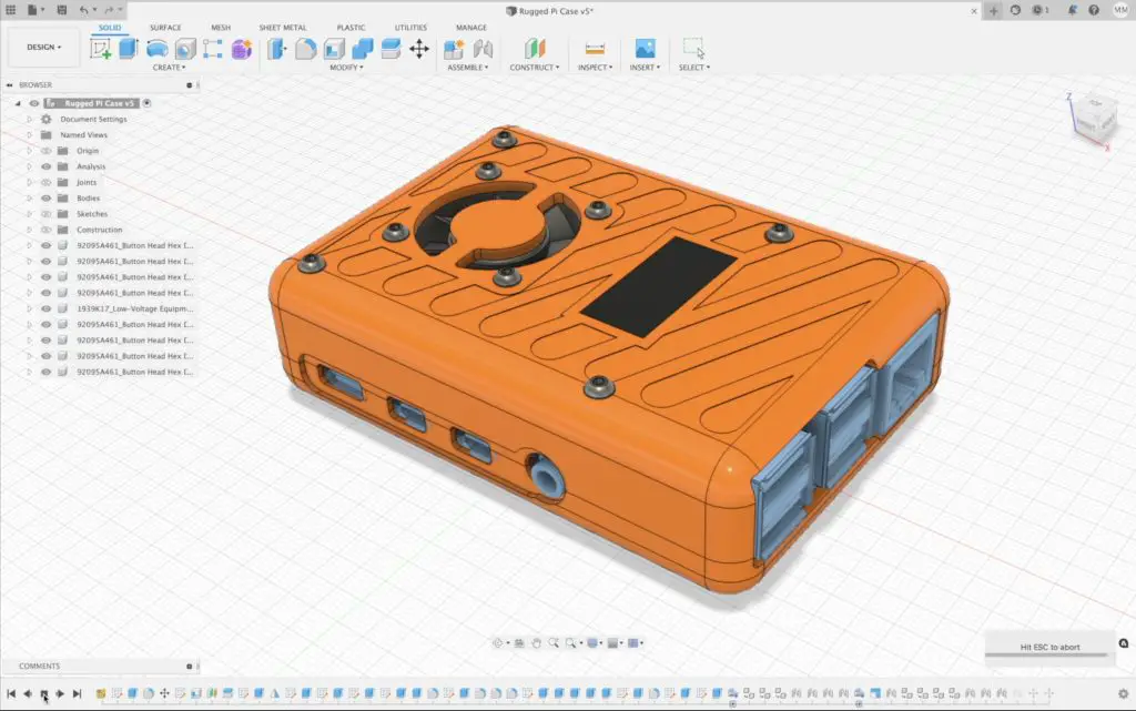
Designing The Home Assistant Hub Housing
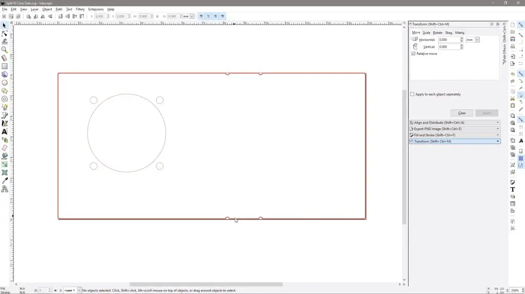
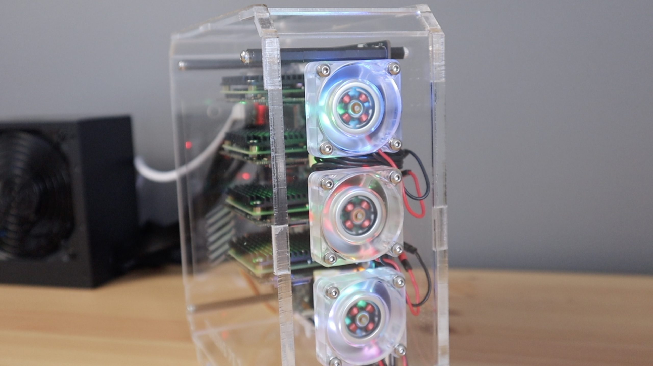
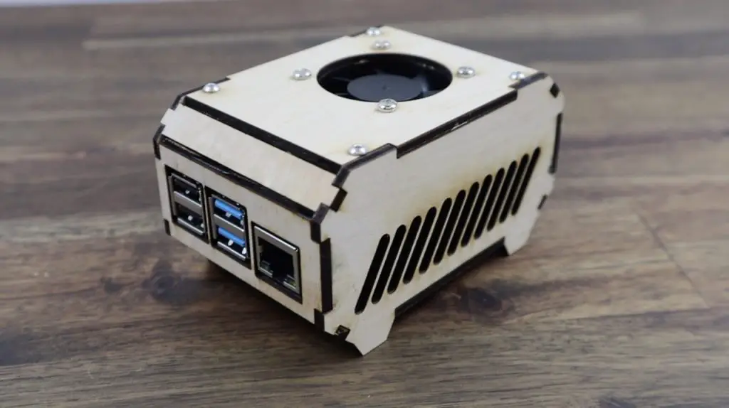
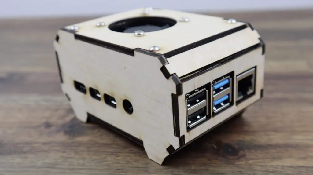
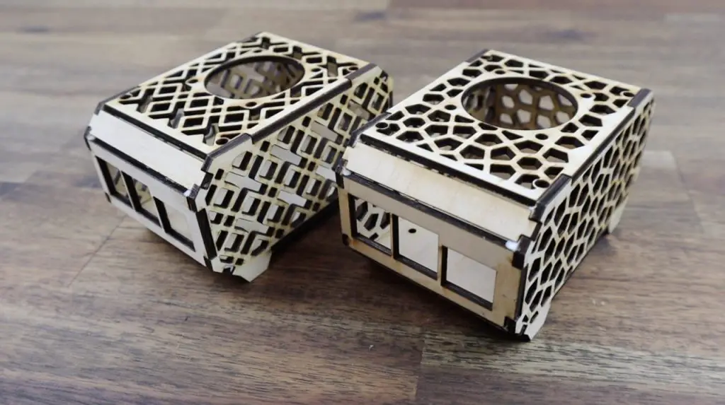
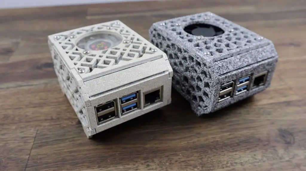
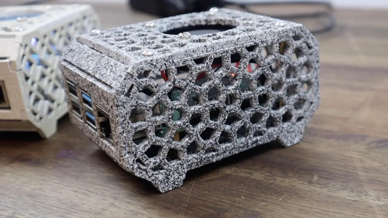
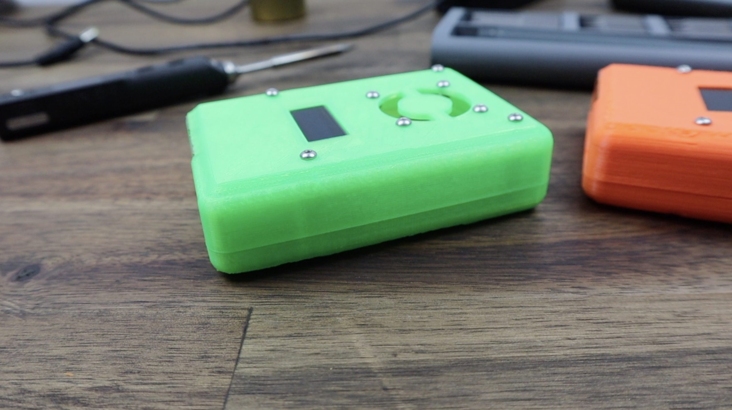
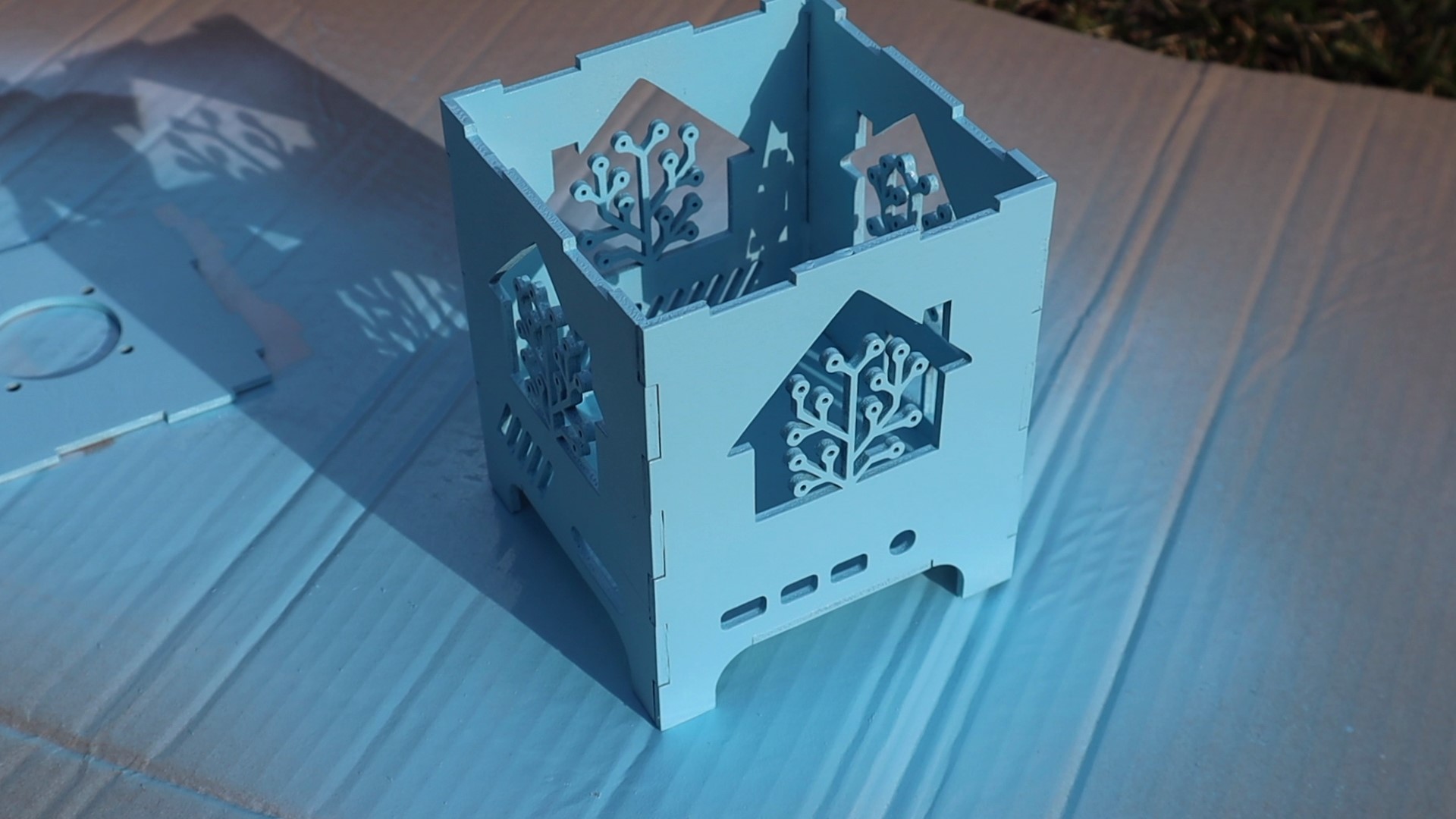
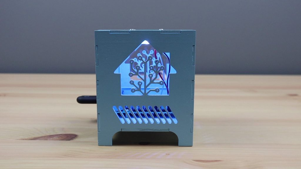
I’ve sketched up a cubic style housing with some feet to lift the Pi off the shelf or desk and a fan on the top for cooling.
Take a look at my video on how to design your own Pi cases in Inkscape.
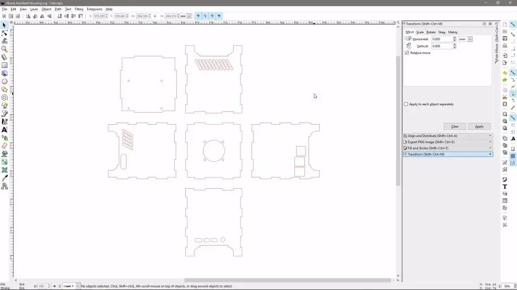
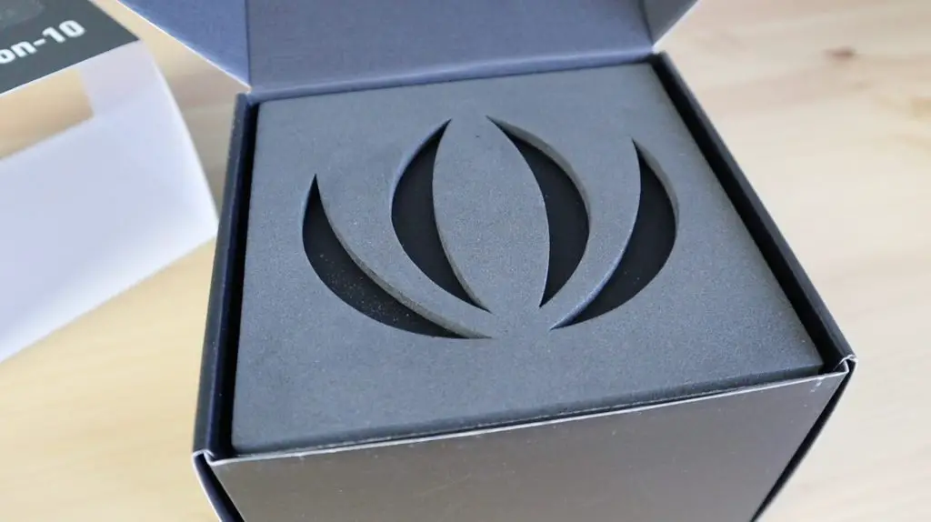
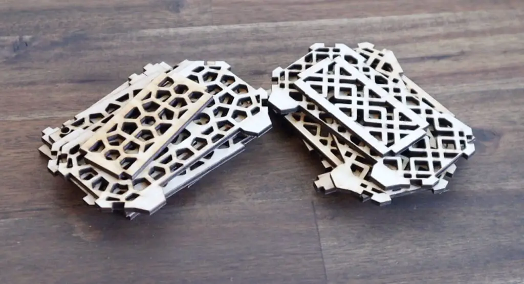
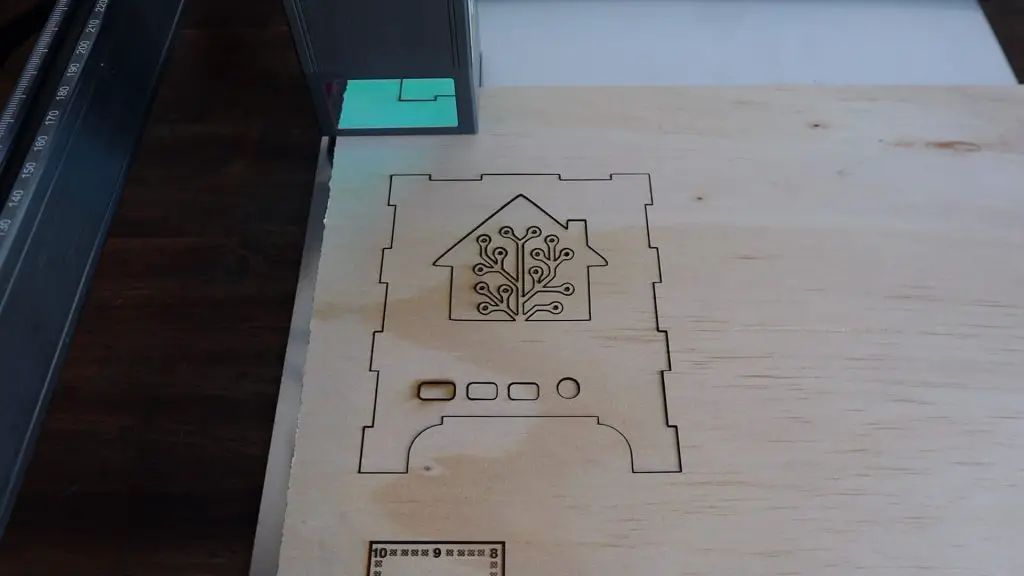
I wanted to integrate the Home Assistant logo into the design in some way, so I initially planned on engraving it. That made the housing look a bit too much like an ordinary box, so I decided to rather laser cut the logo out on each side.
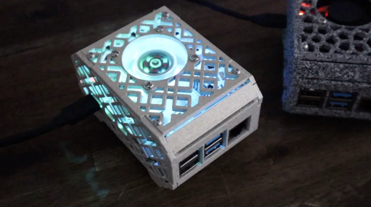
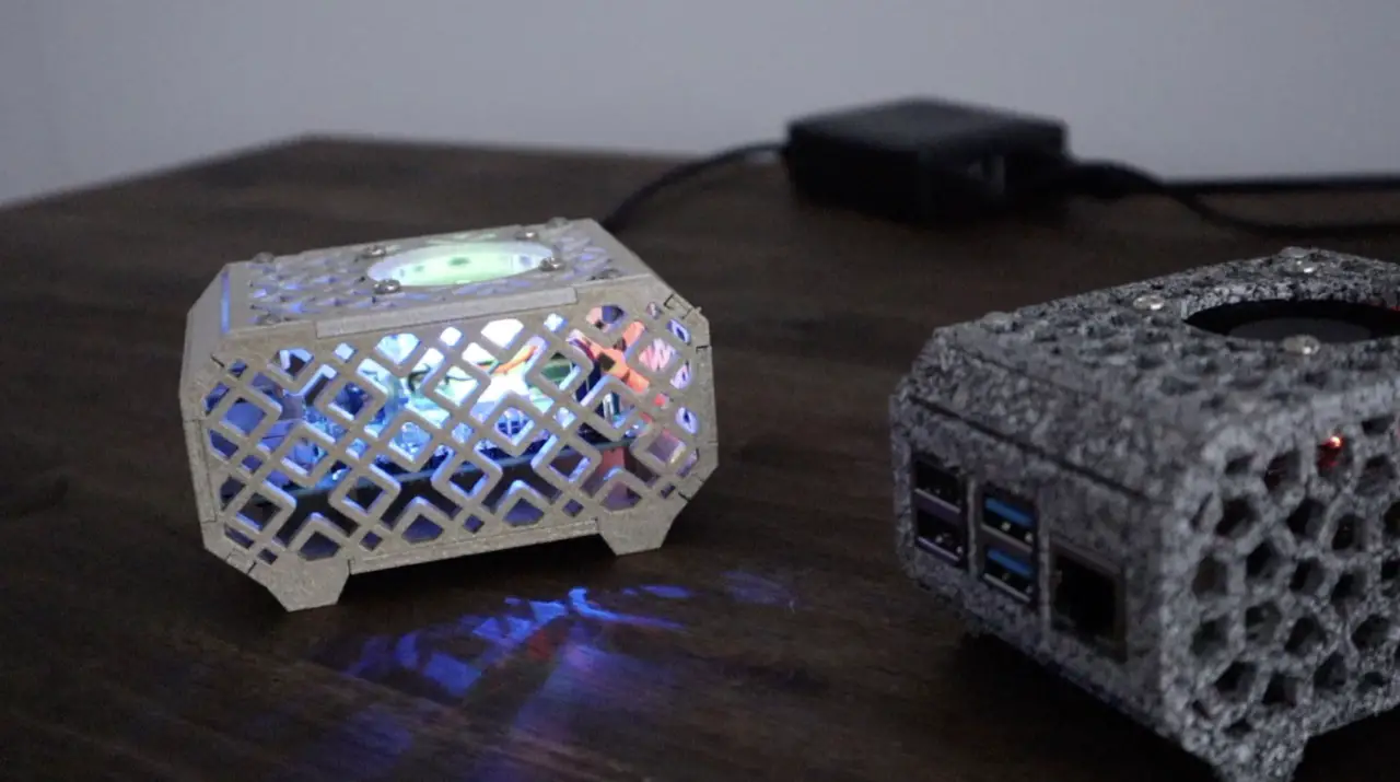
I can then glue some clear acrylic or clear plastic sheets onto the inside of the case to keep the dust out. The RGB lighting on the fan should light up the inside of the case just enough to give the logo a bit of a glow – which will hopefully look quite good.
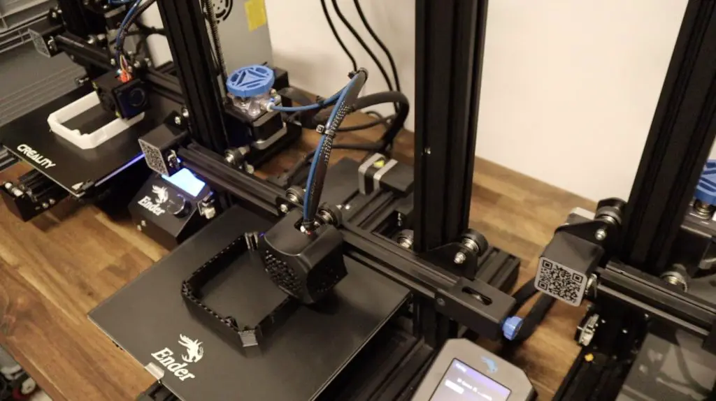
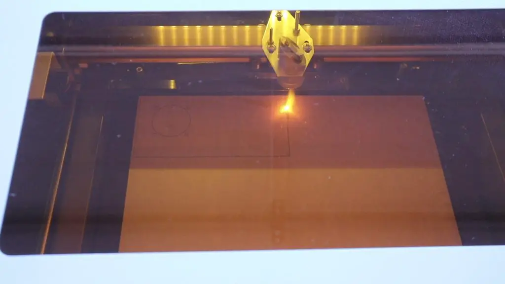
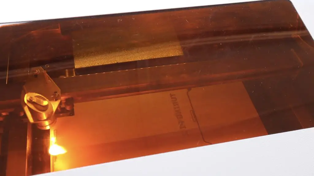
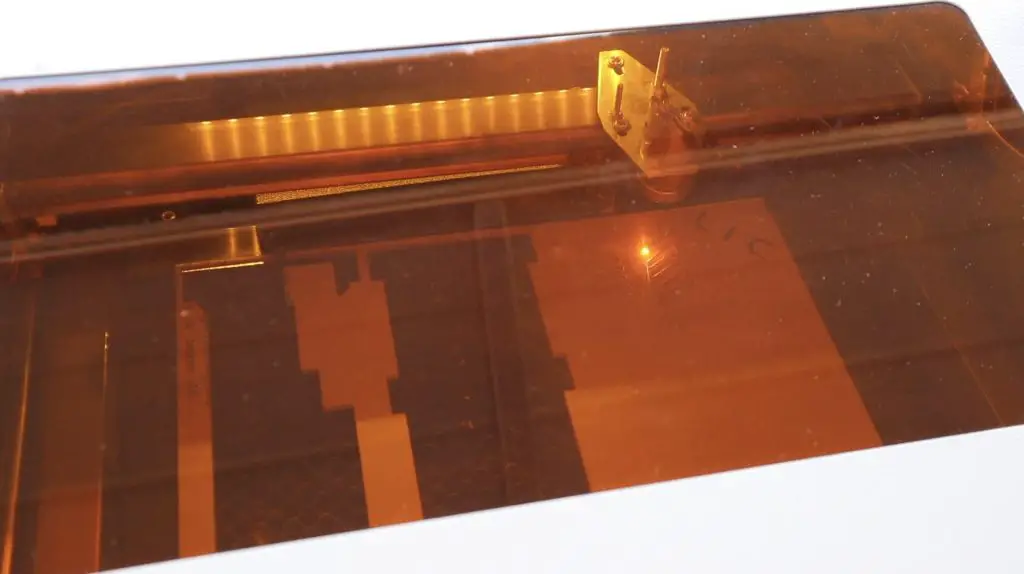
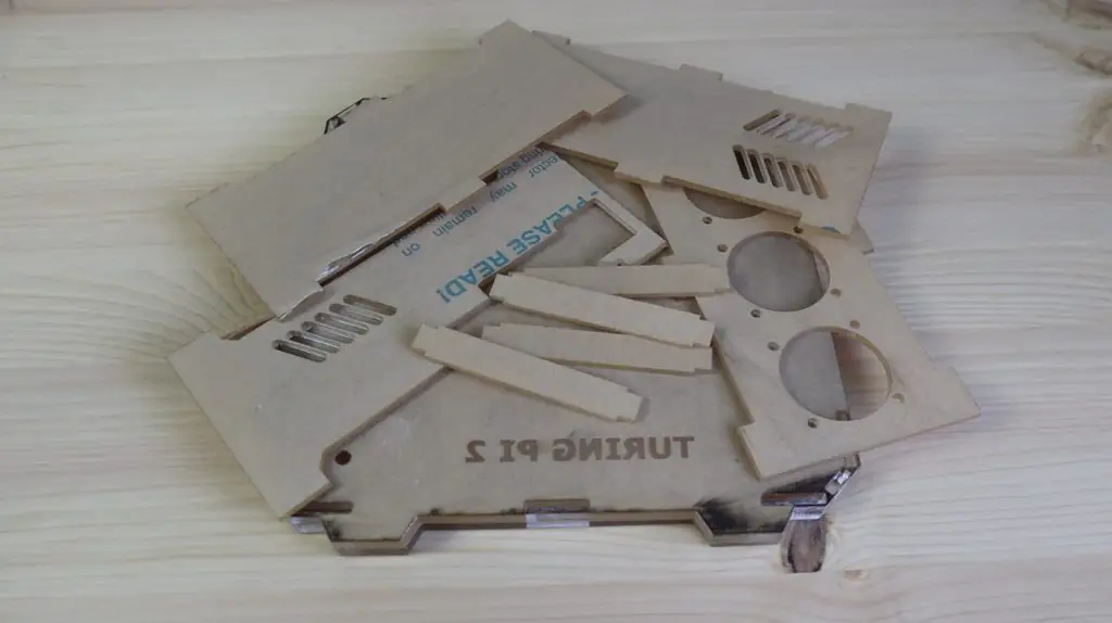
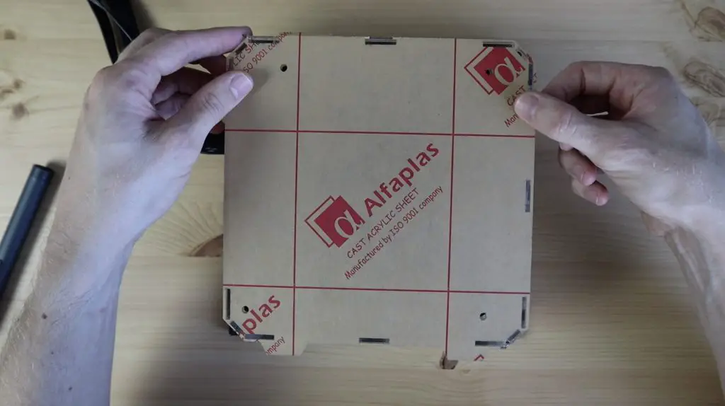
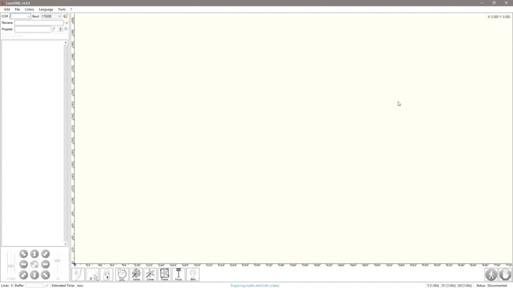
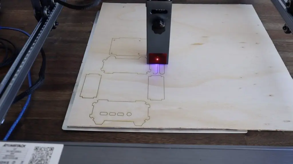
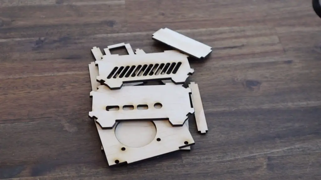
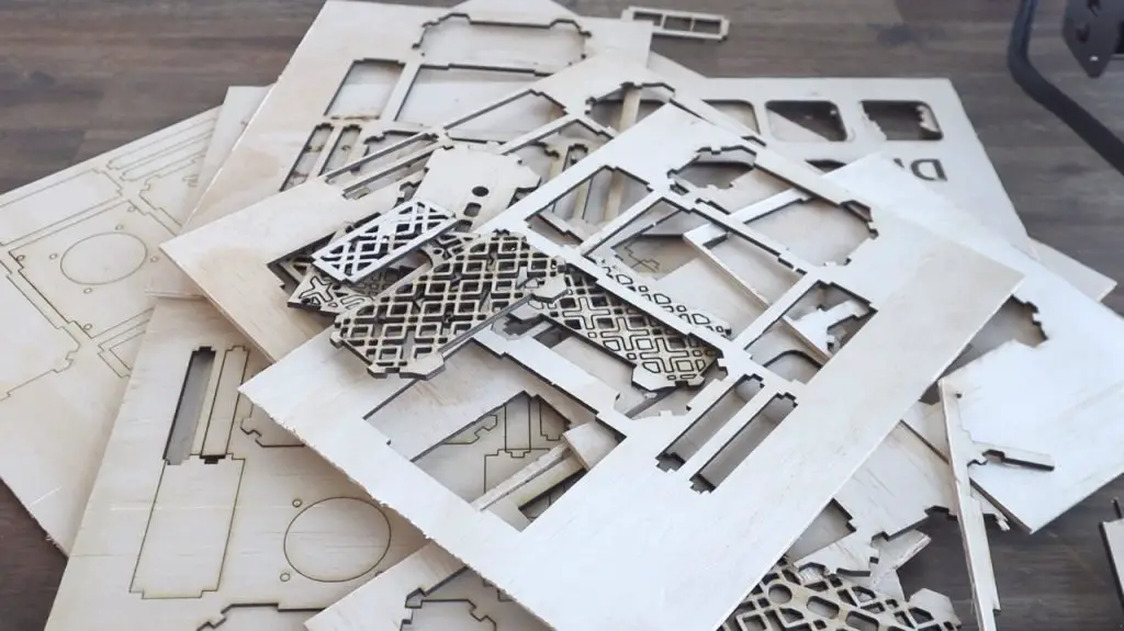
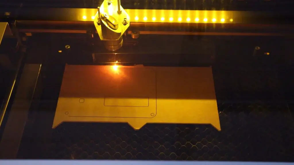
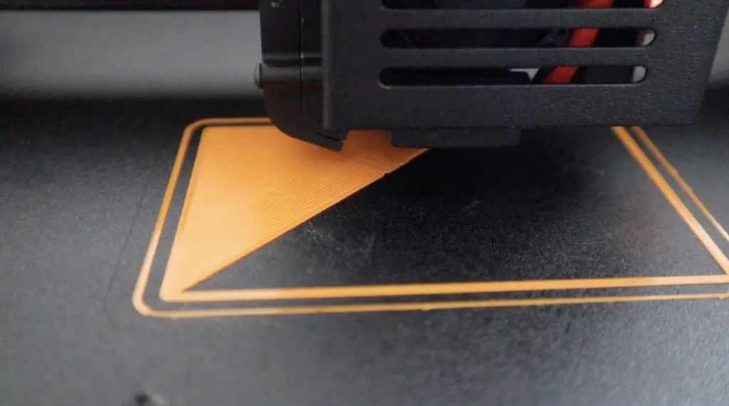
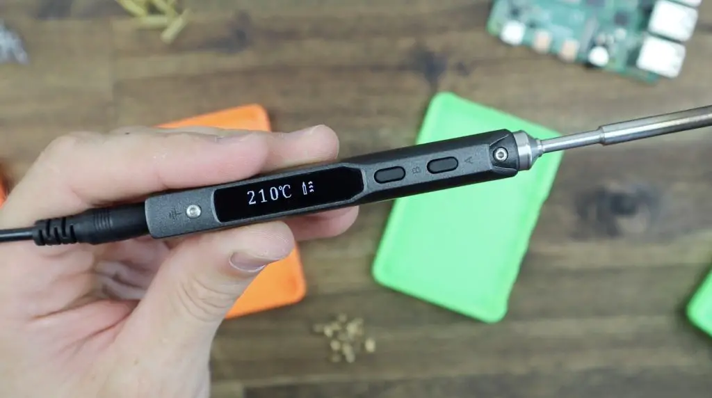
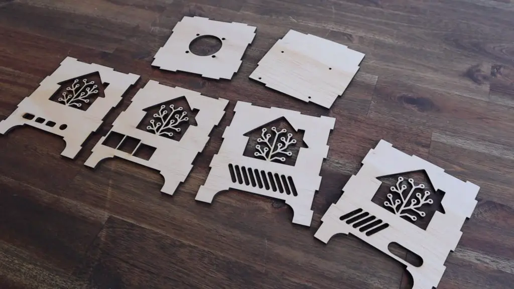
Let’s get the components cut on the Atomstack X20 Pro. I’m going to be cutting the components from the same sheet of 3mm plywood. I’m cutting at 300mm/min and 90% power. I’ve prepared the files in laserGRBL and I’m going to again use the microSD card and offline controller to do the actual cutting. I find this easier than having to set up a laptop near the laser.
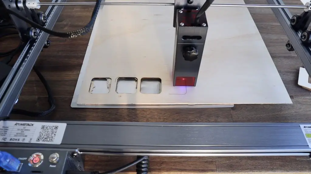
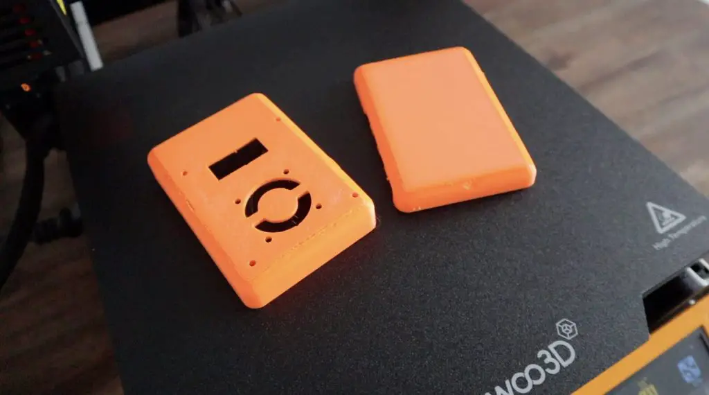
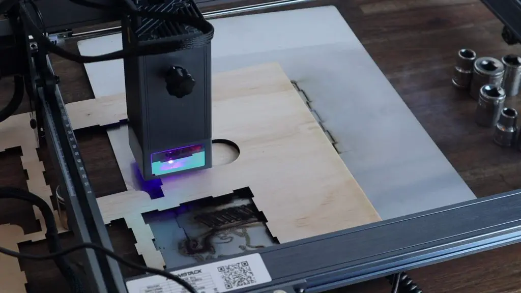
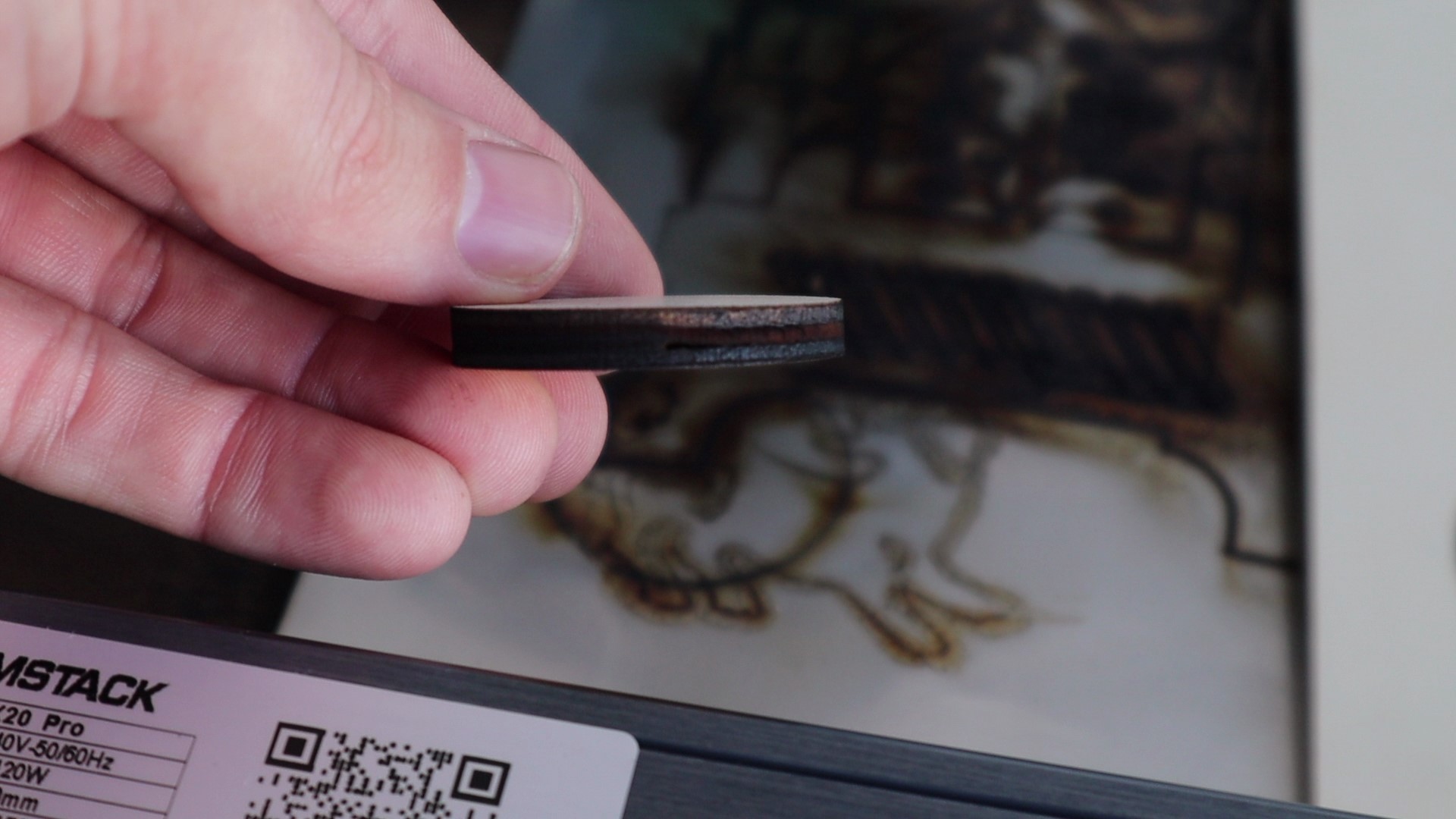
The first piece came out perfectly and you can really see how the air assist has helped to keep the smoke away from the plywood. I started without it for the first USB C port cutout and you can see it’s surrounded by smoke stains. I then turned the air assist on to about 30% power and the rest of the cuts are really clean on the surface.
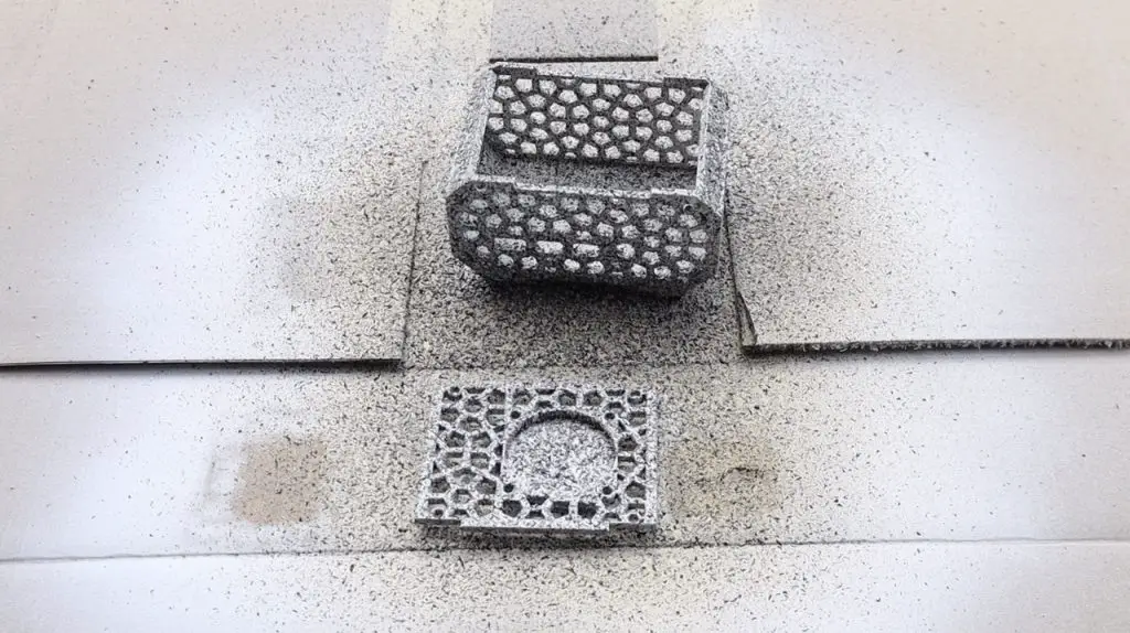
The underside gets marked from some of the reflected laser’s light, so I’ll probably look at adding a honeycomb bed at some stage. I also noticed that the localised heat from the laser caused pretty significant warping on the metal sheet once all of the pieces had been cut.
One thing that is a bit of an issue with all of these diode lasers is that there is no smoke extraction system, and cutting wood produces a lot of smoke. So you need to work in a well ventilated area.
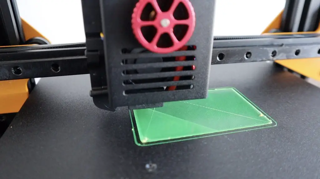
Just as a test, I tried a piece of 6mm plywood that I had lying around. I set the laser to 200mm/min and 100% power and it had no problem cutting this out in a single pass either.
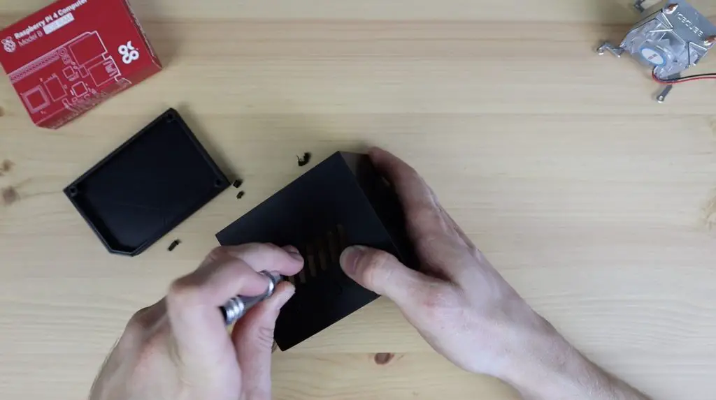
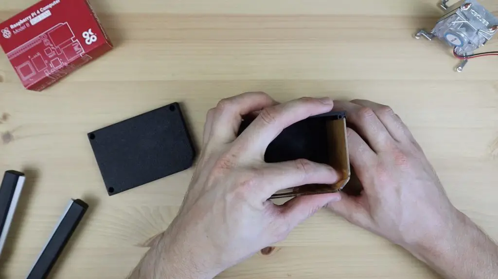
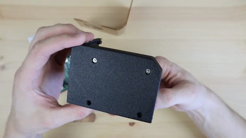
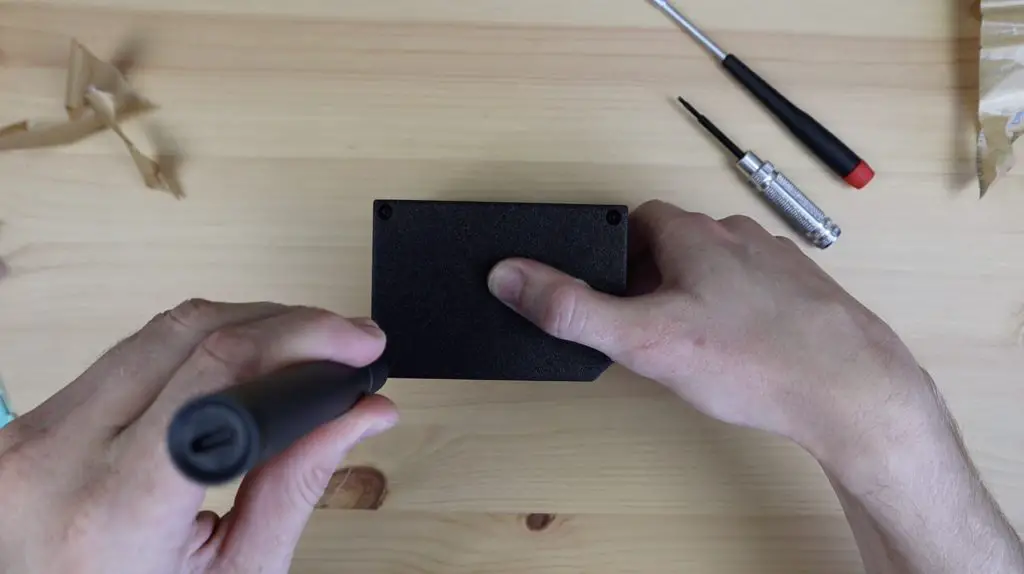
Assembling & Painting The Hub Housing
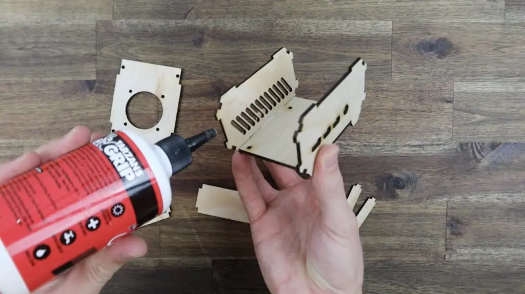
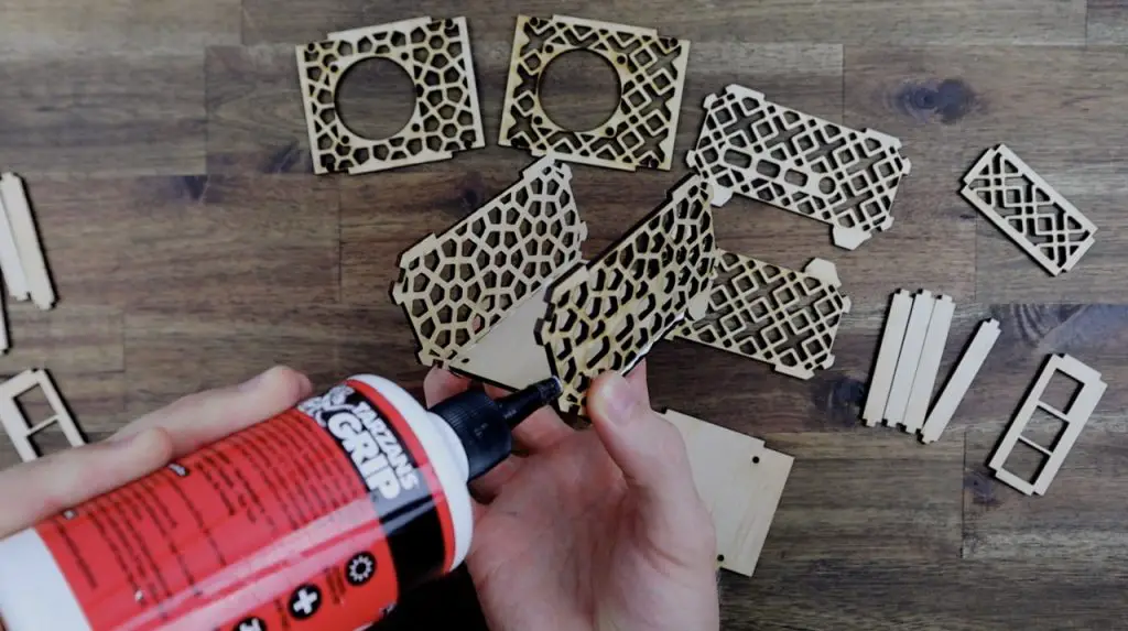
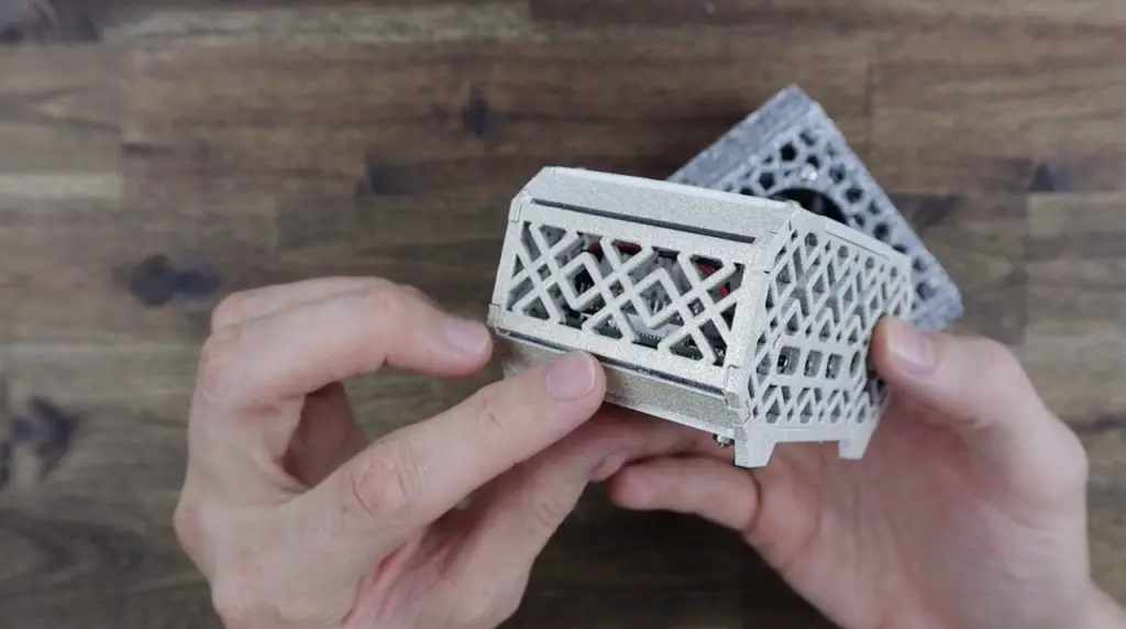
Now that we’ve got the pieces cut out, lets glue them together and give the housing a light sand.
I’m just going to use regular PVA wood glue to glue it together and then I’ll leave it to dry for a few hours before sanding it.
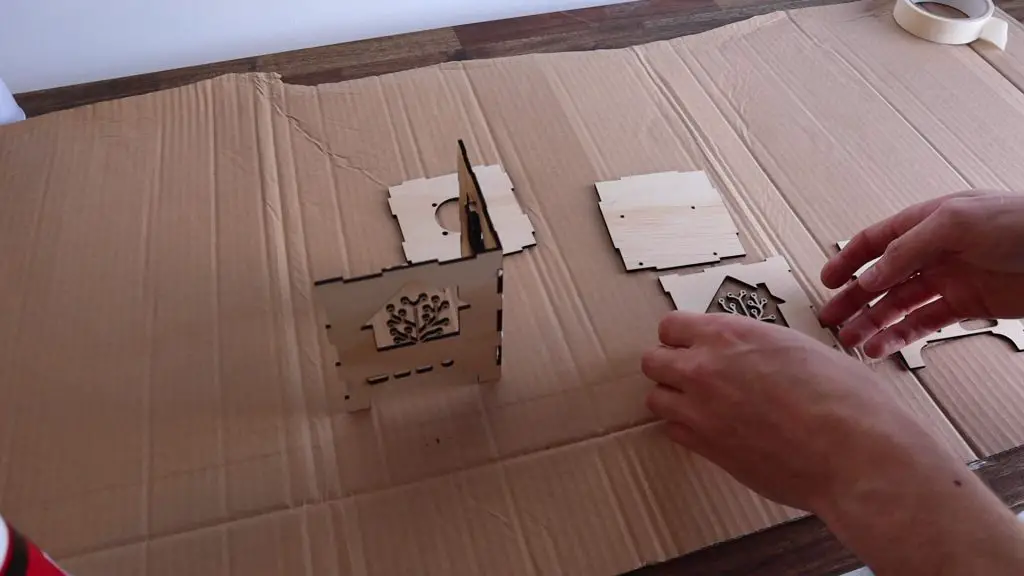
I used a couple of strips of masking tape to hold the sides together while the glue dried.
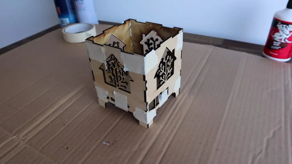
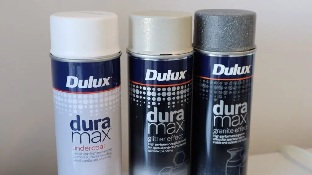
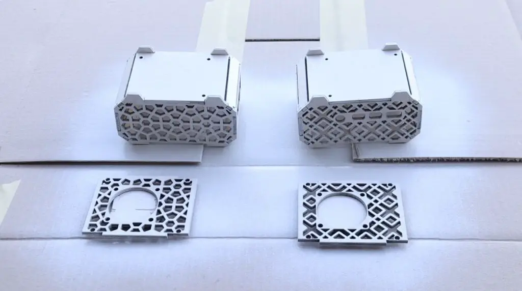
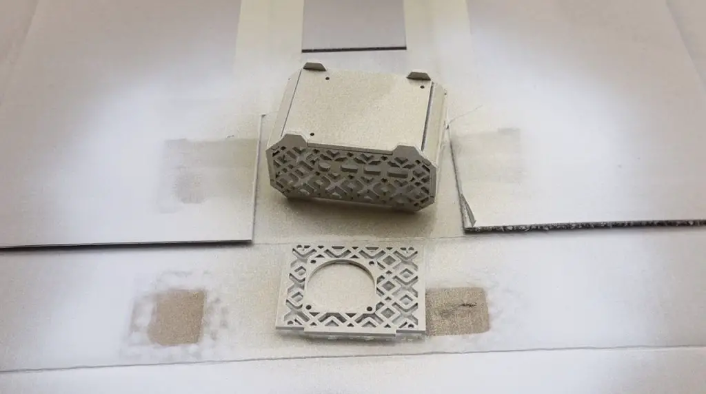
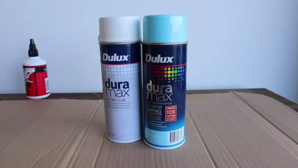
I’m going to paint the housing with two coats of a white universal undercoat and then two colour coats. I couldn’t find the exact colour of the Home Assistant logo, but this colour (called Fish Pond for some reason) is about as close as I could find – so I’m going to try it out and see what it looks like.
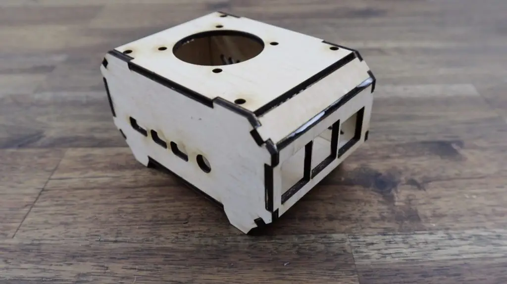
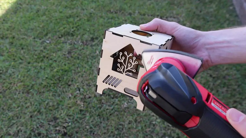
Once the glue was dry I gave the corners, edges and faces a light sand with 240 grit sandpaper.
I then painted the housing with the two coats of undercoat and two coats of enamel paint, allowing each coat to try for about half an hour before applying the next one.
After a second colour coat, it’s starting to look pretty good. I just want to fill in the edges a little more and it’ll then be done.
Engraving the Lid Using the X20 Pro’s App
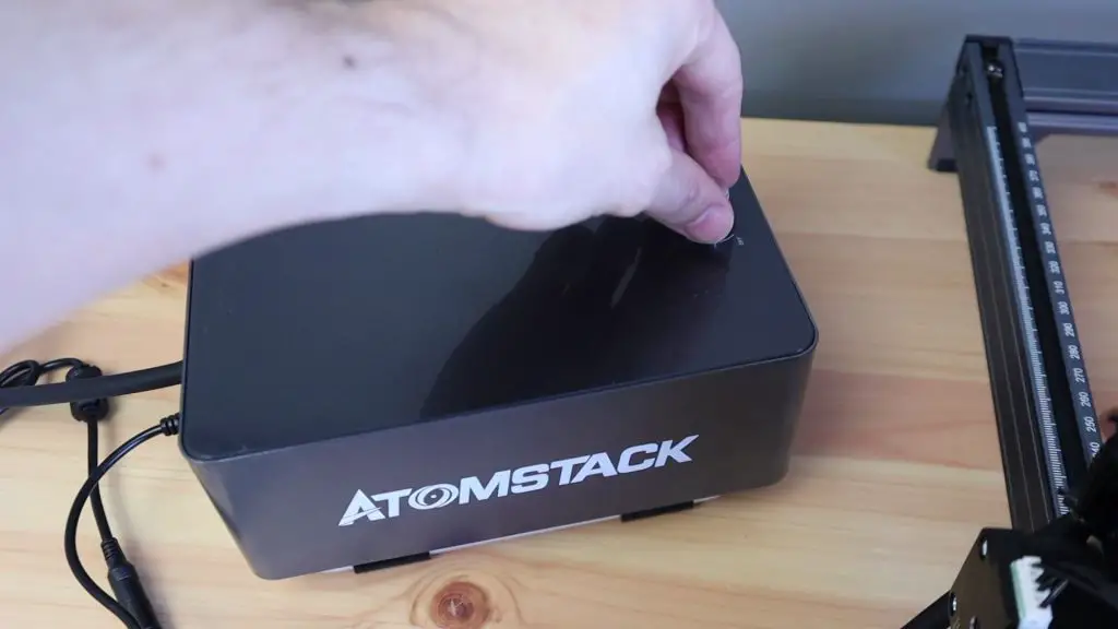
Atomstack have also added an app on the software side that allows you to quickly import and engrave or cut shapes, sketches and images wirelessly, which is great to improve your workflows.
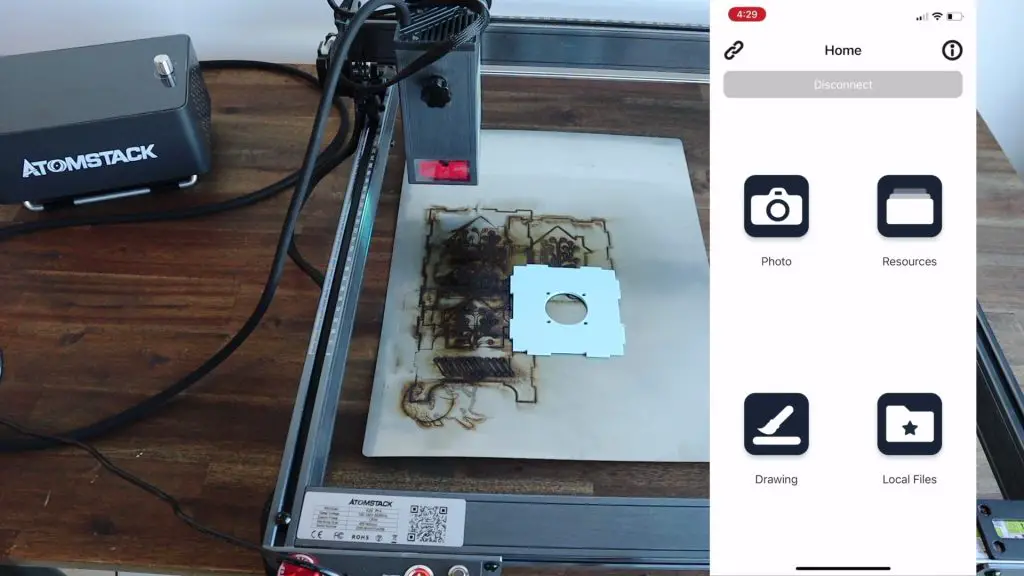
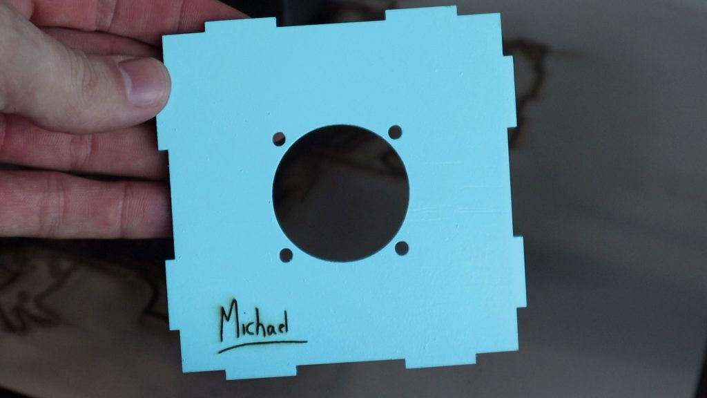
So I’m going to try and use the app to add some text to the lid of the housing. I’m going to quickly sketch my name in the app’s freehand editor and then engrave it onto the lid.
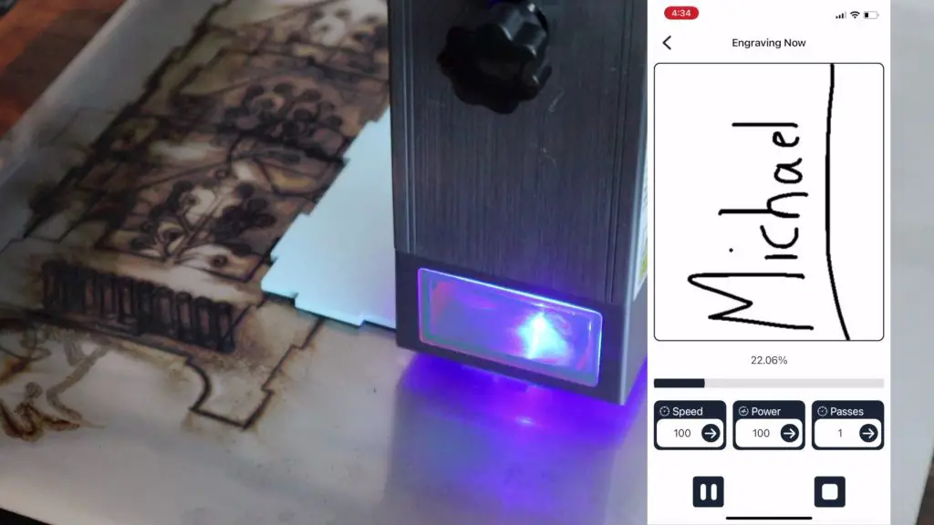
The app definitely has its limitations, but it’s a great way to quickly add details to pieces where accuracy isn’t particularly important. For anything important, I’d probably still resort to using my computer or the offline controller to control the laser more accurately.
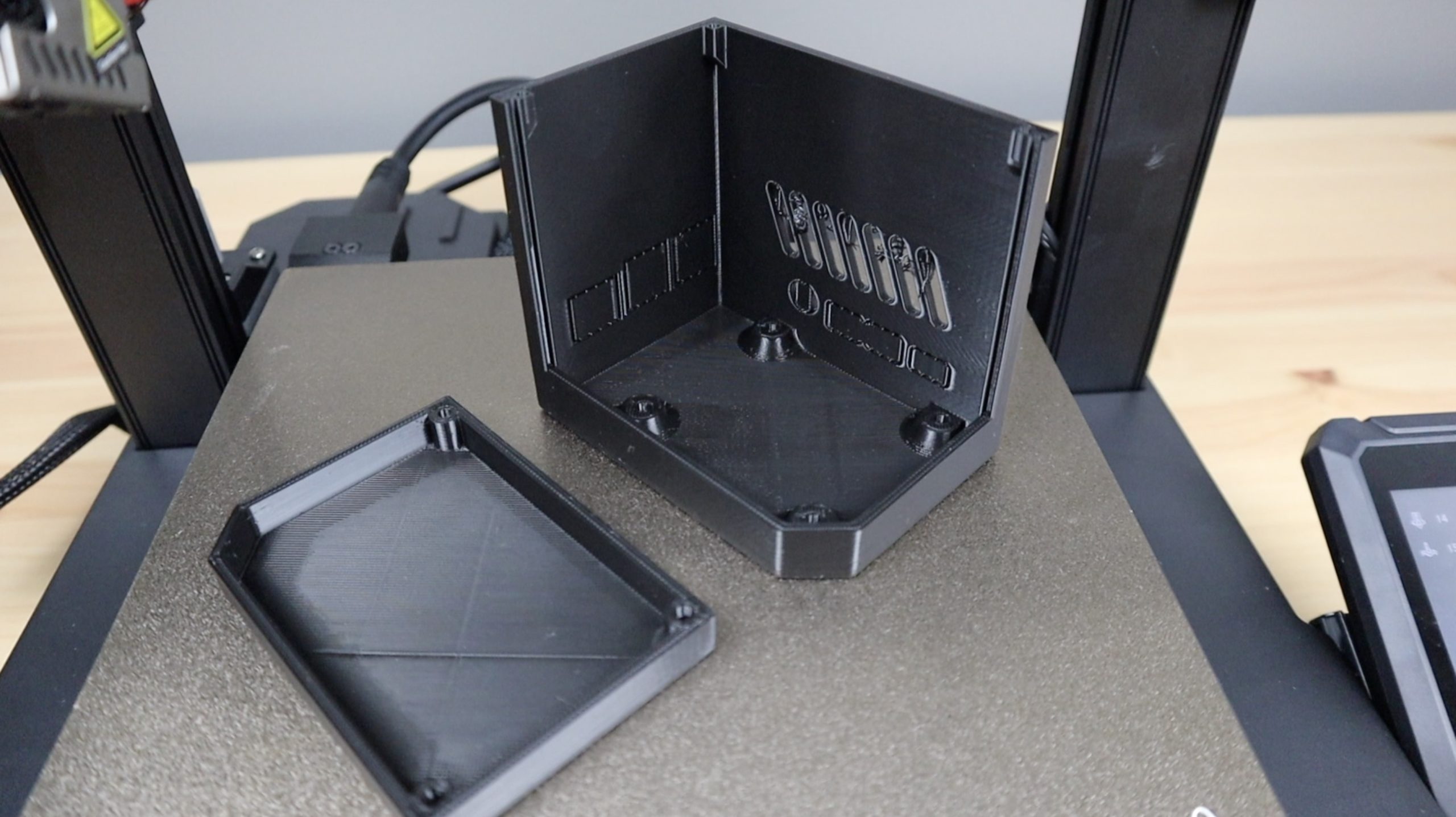
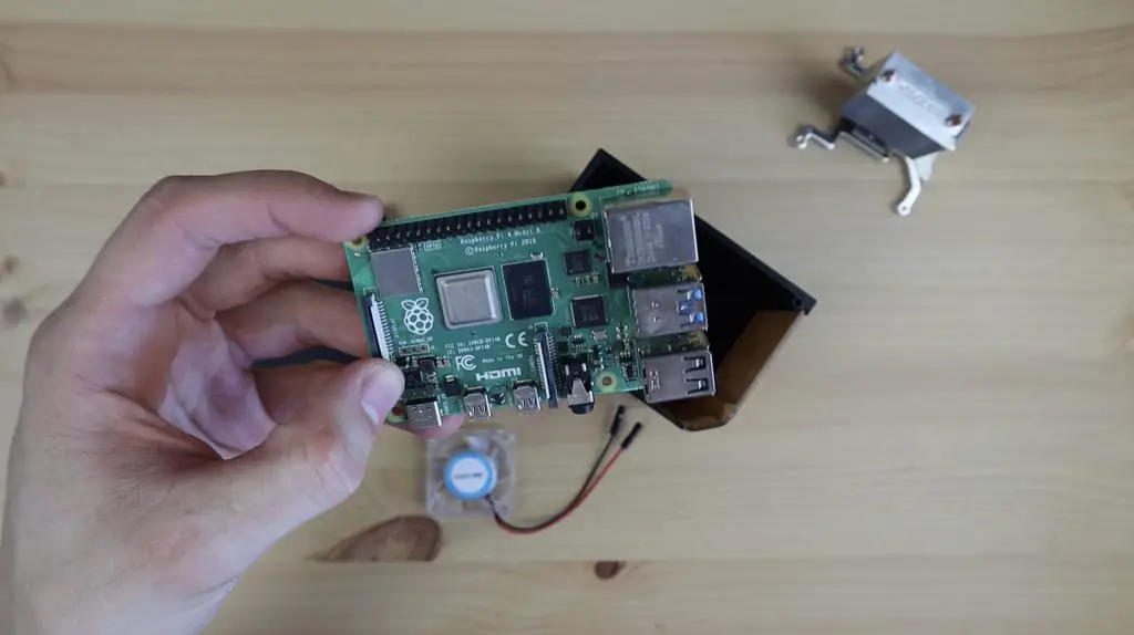
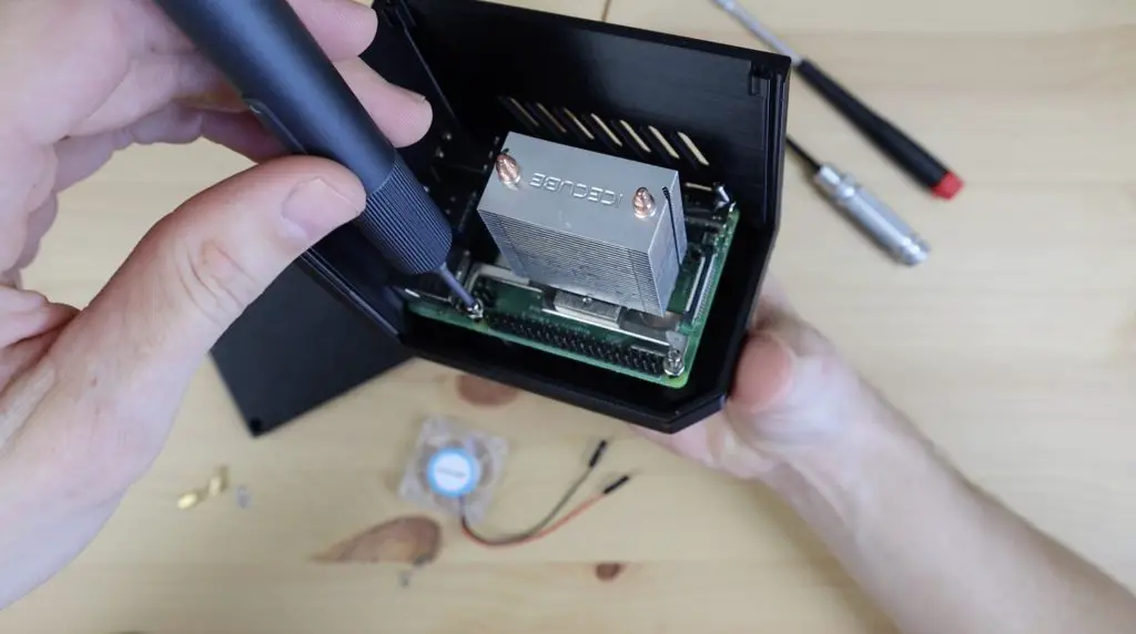
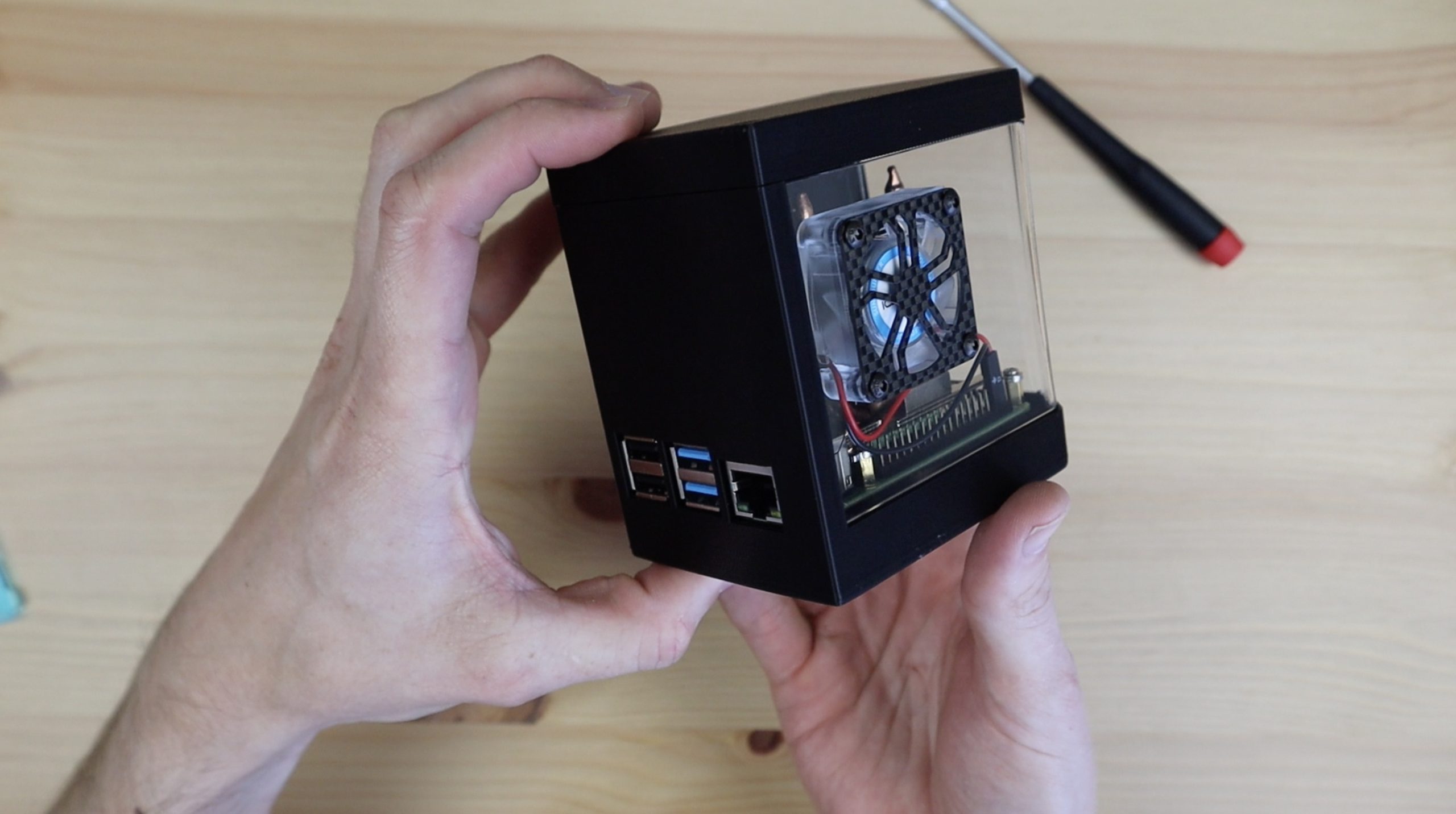
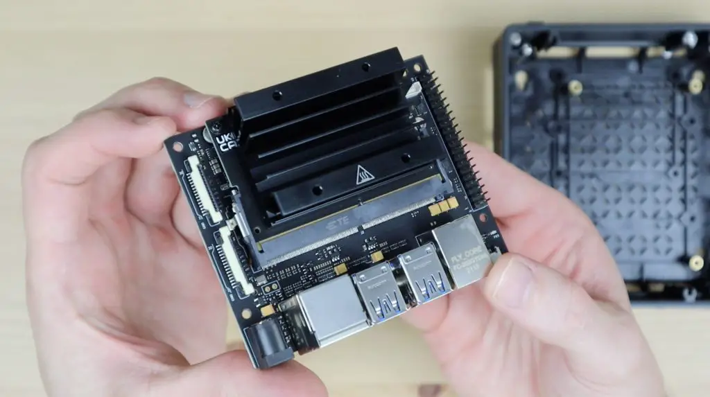
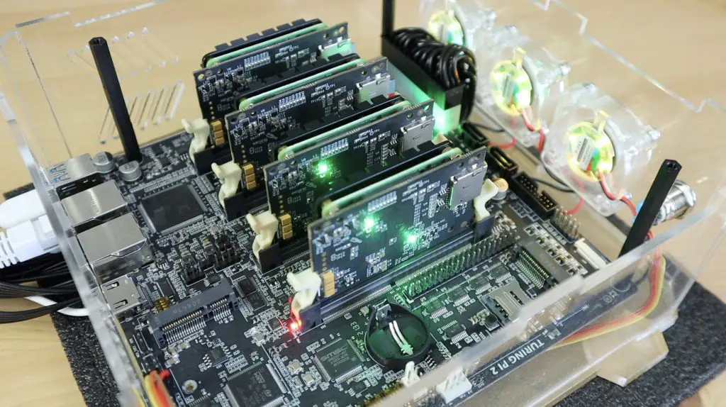
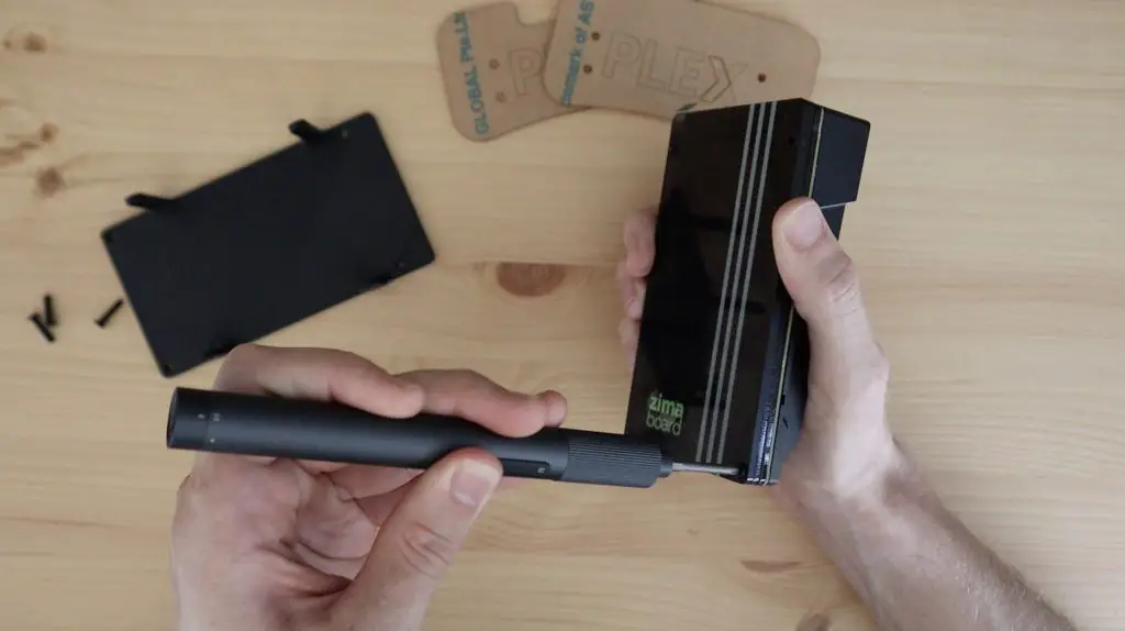
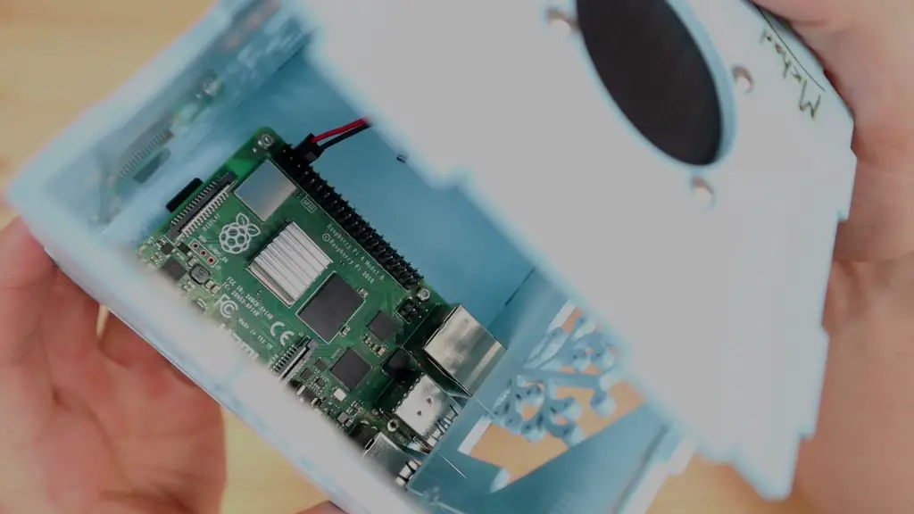
Installing The Home Assistant Hub Electronics
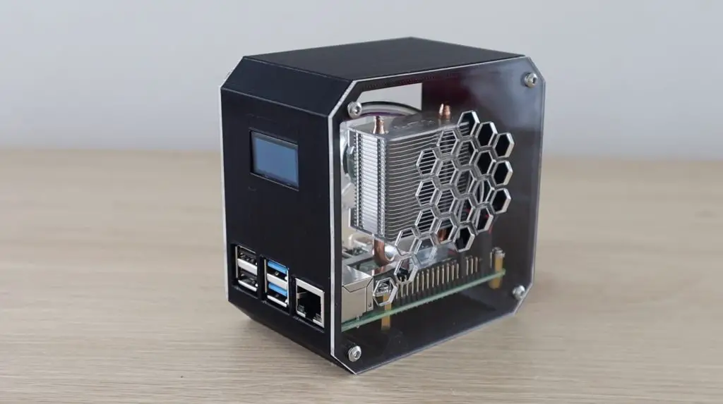
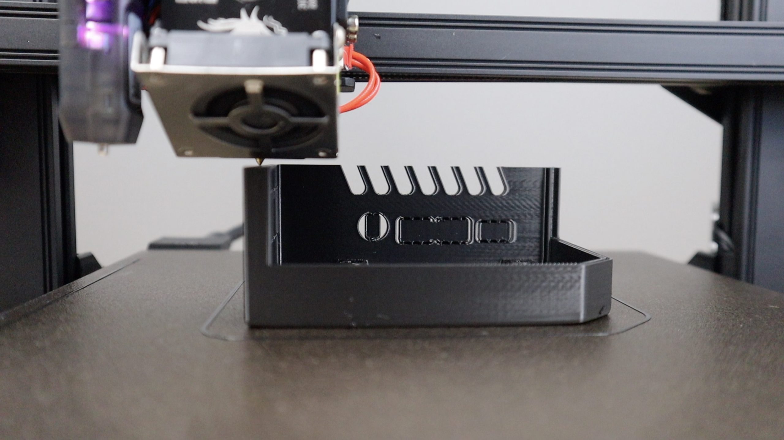
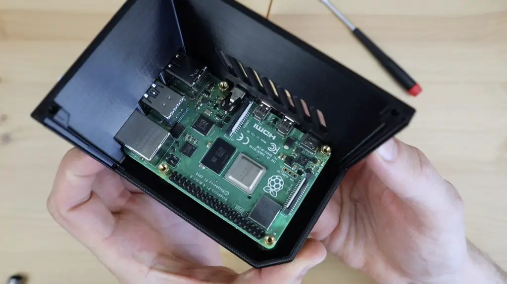
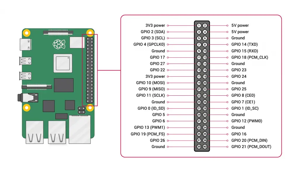
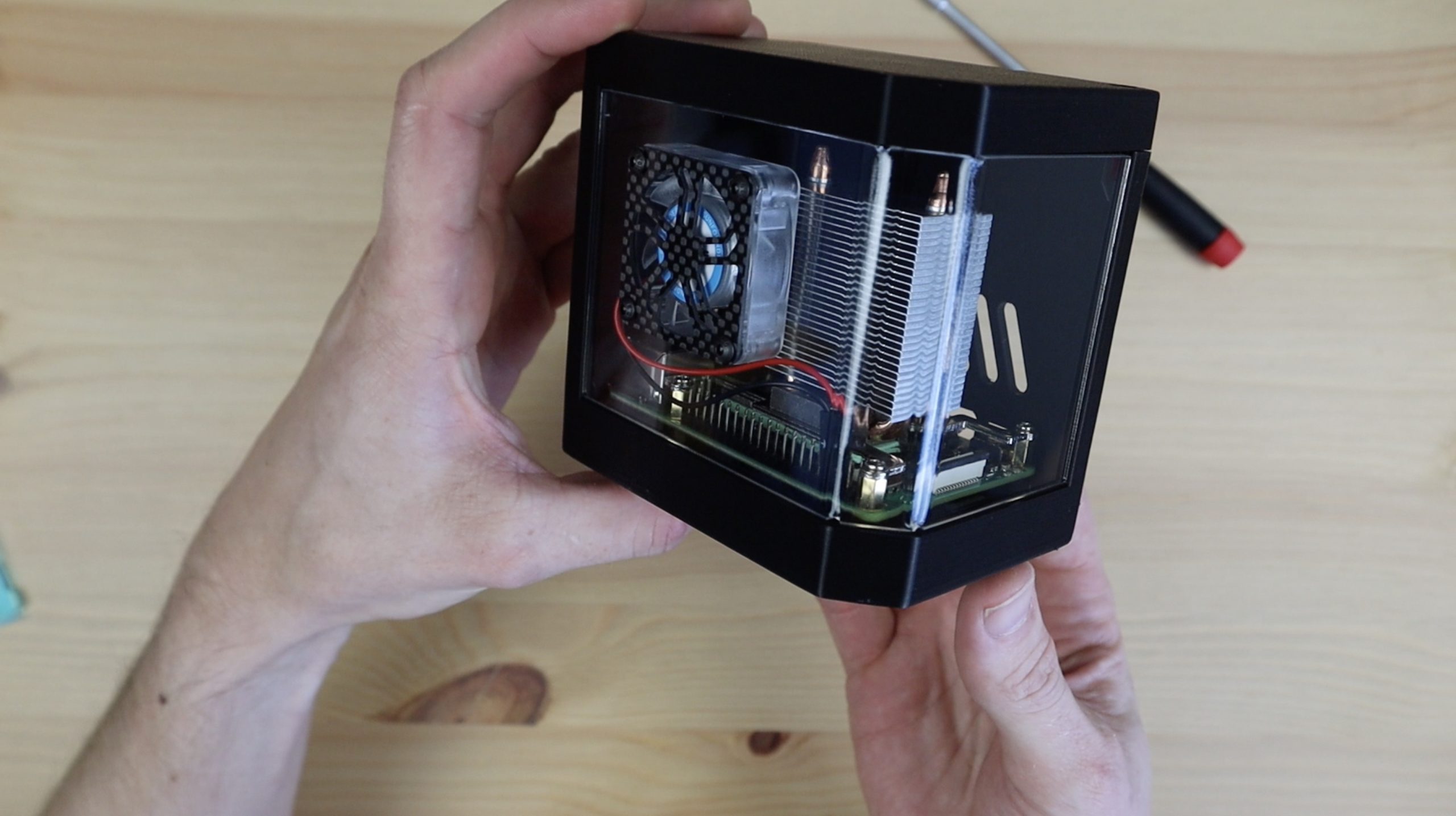
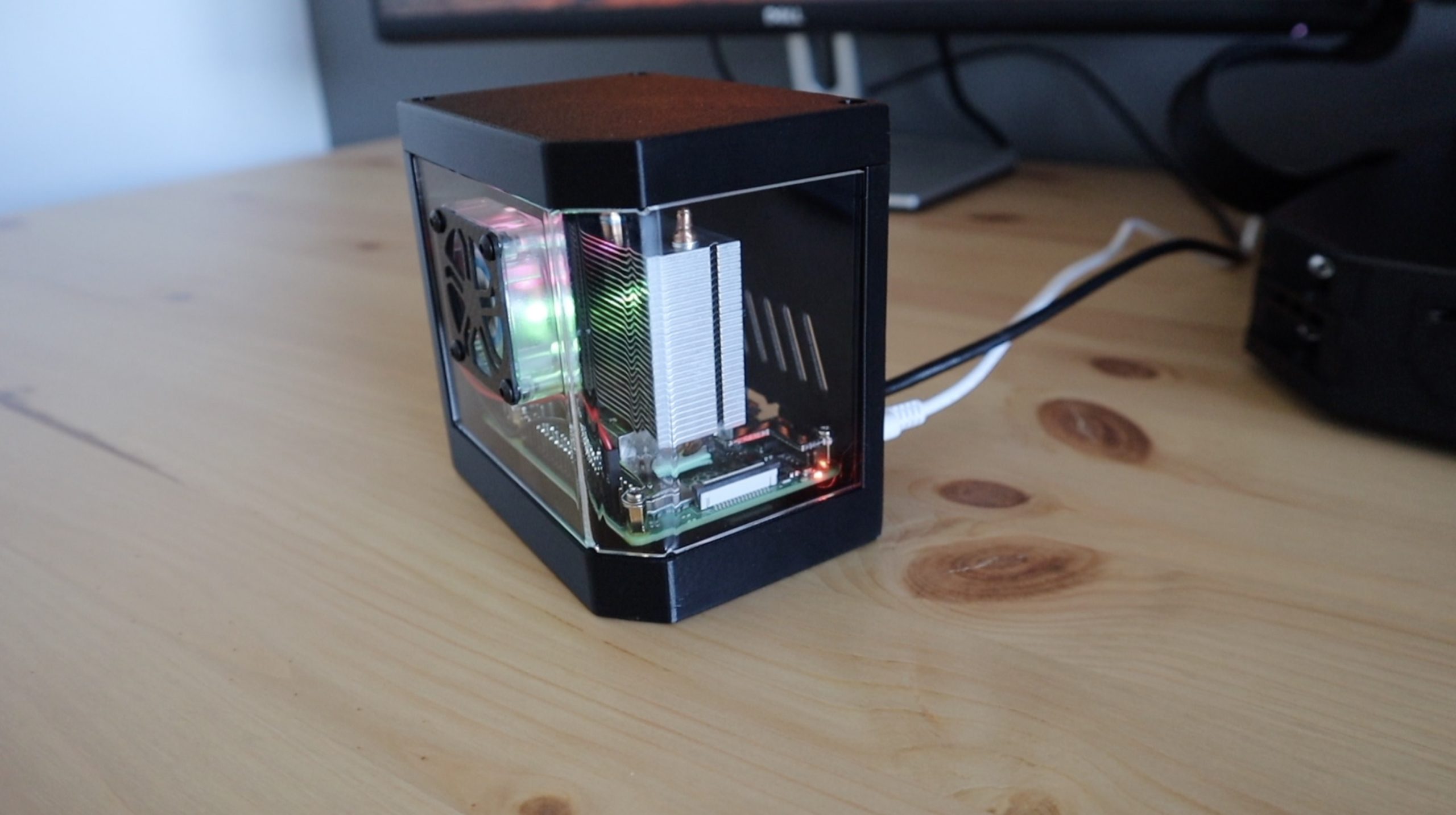
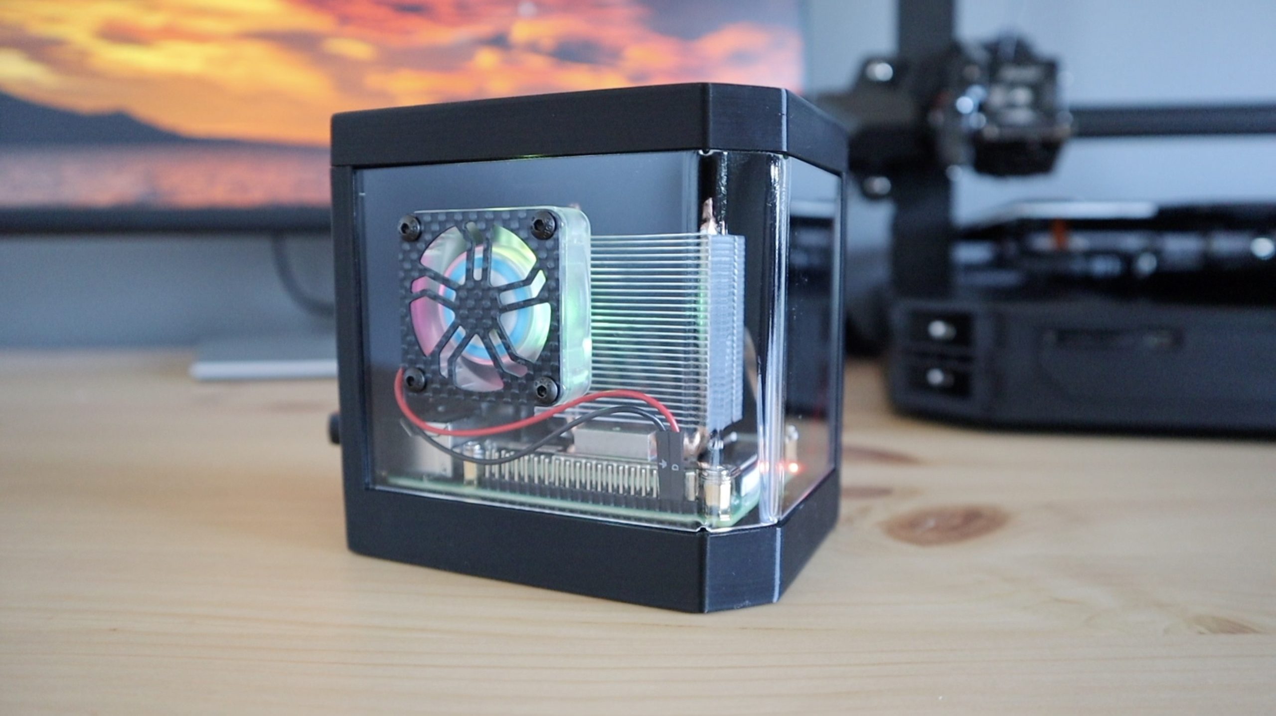
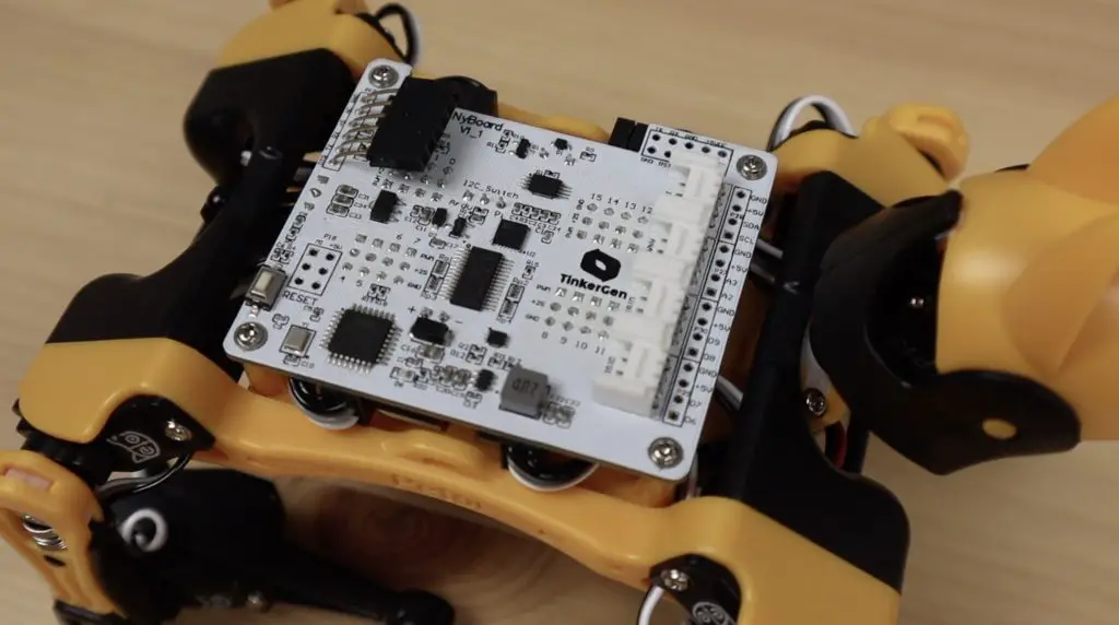
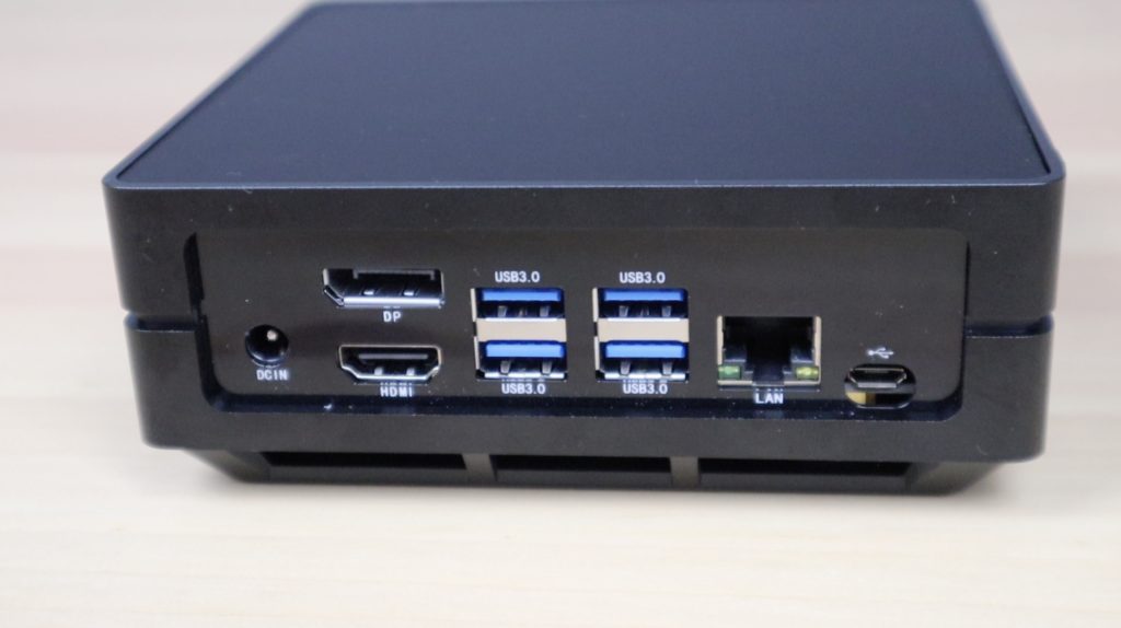
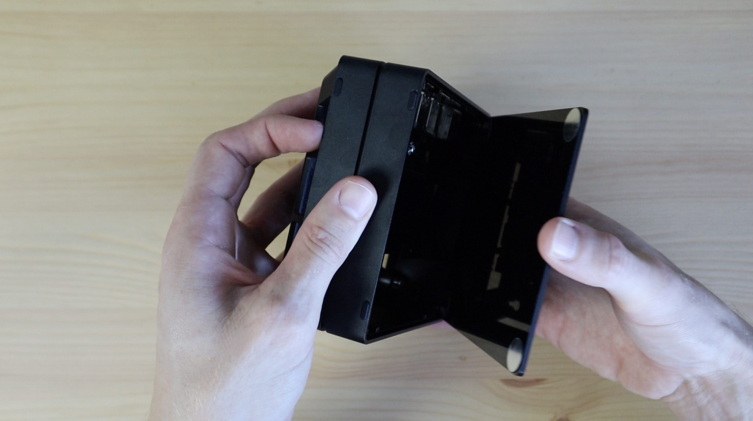
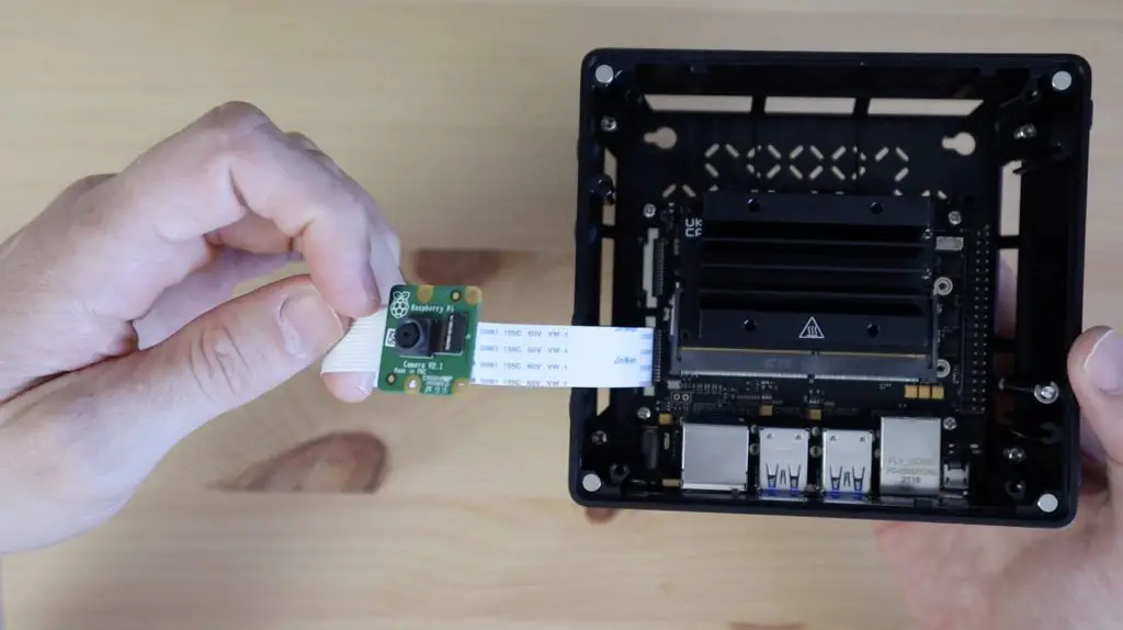
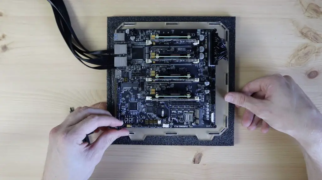
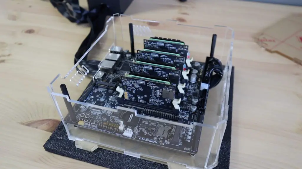
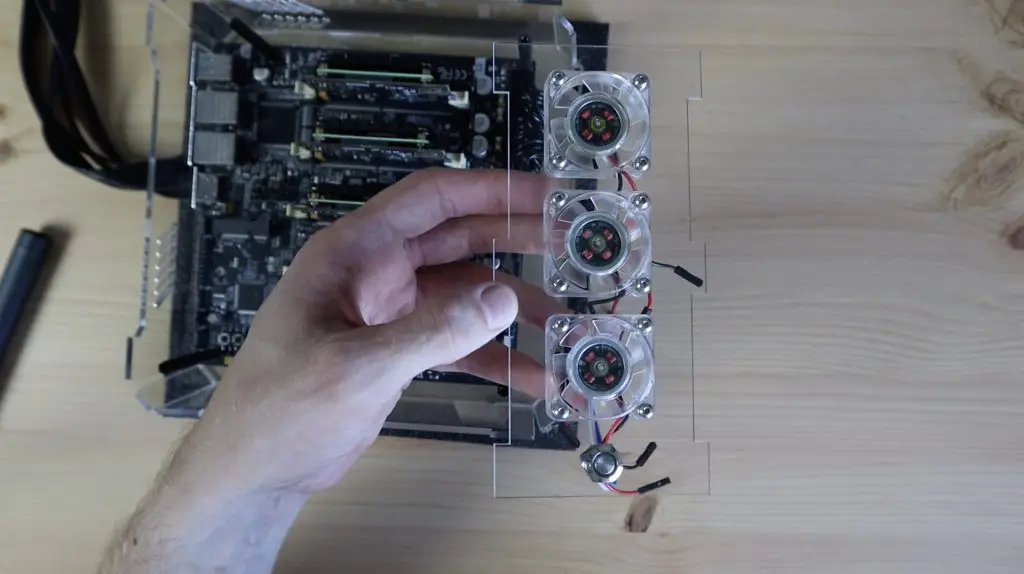
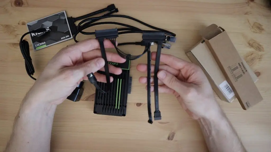
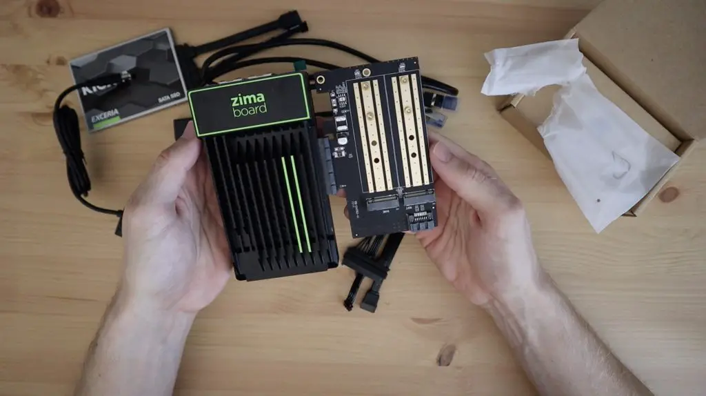
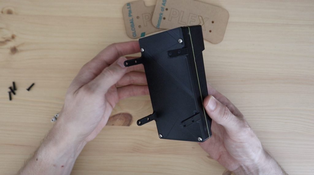
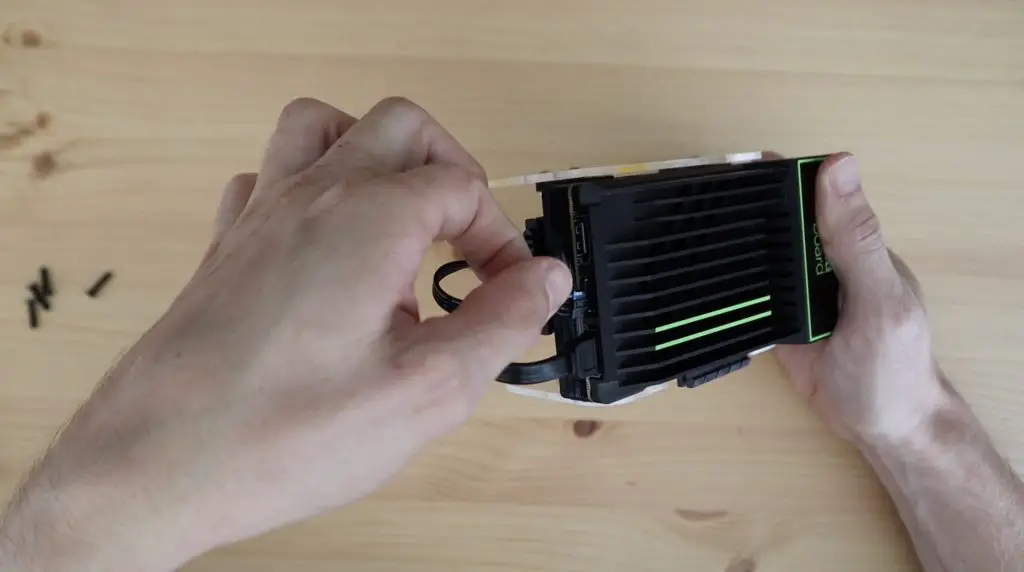
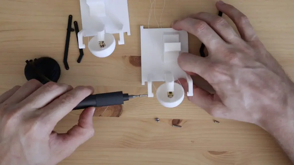
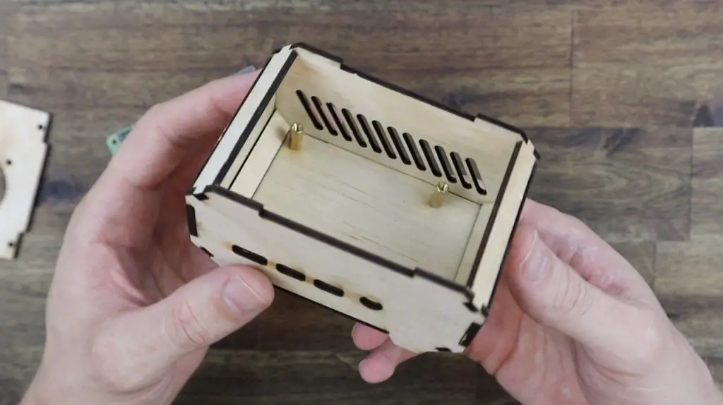
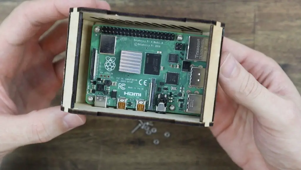
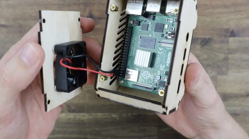
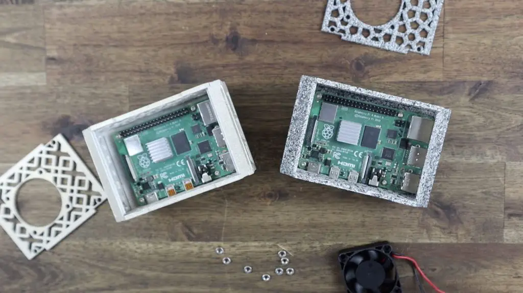
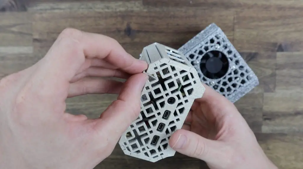
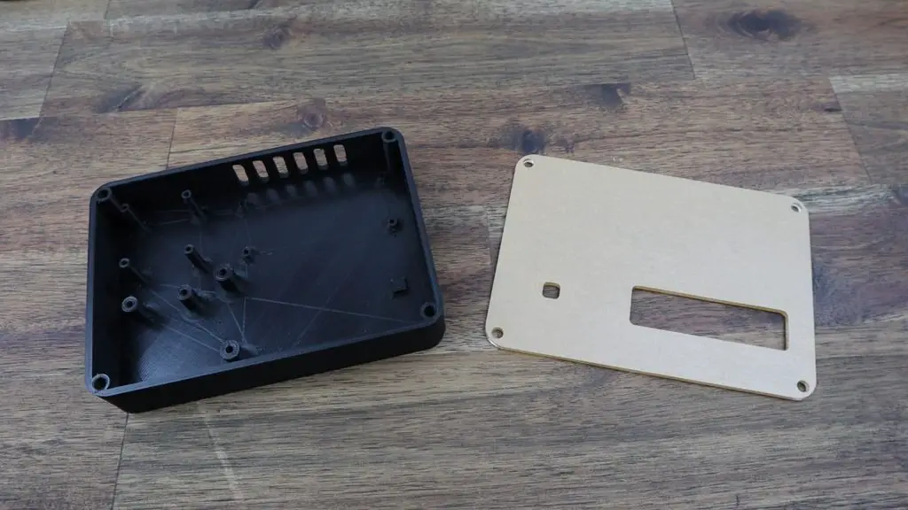
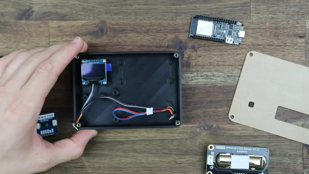
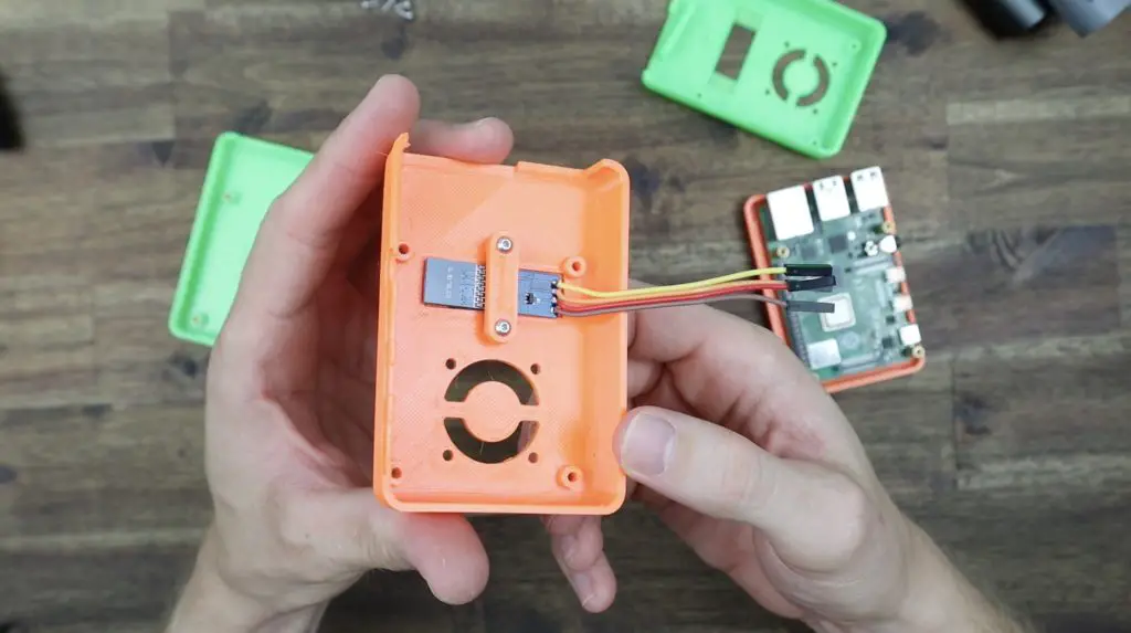
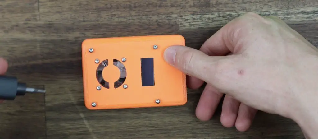
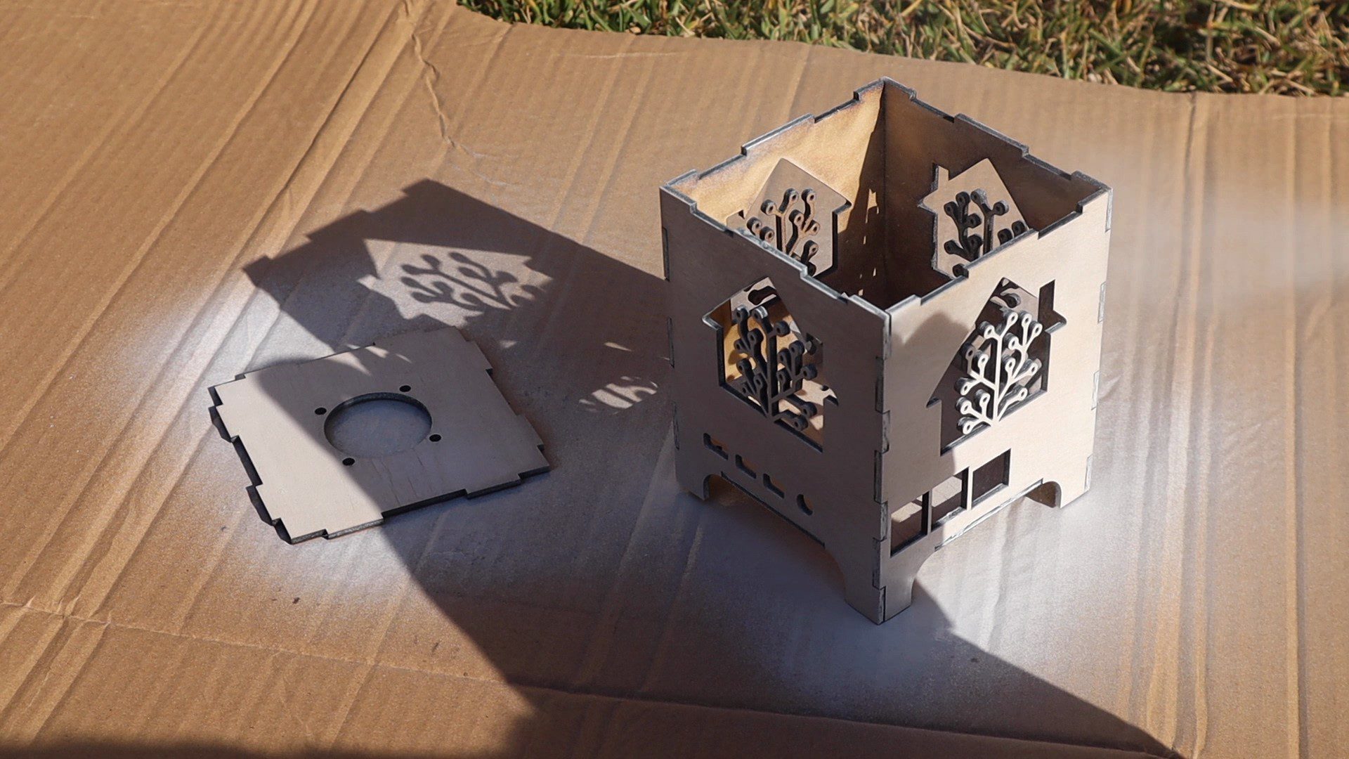
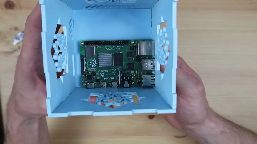
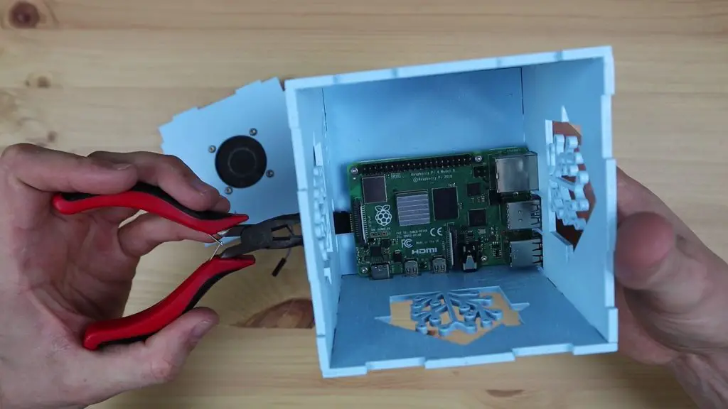
Now let’s get our Pi and fan installed in the housing. I’ve intentionally left a bit of headroom in the top so that there’s space to add shields, adaptors or devices onto the GPIO pins in future as I need them.
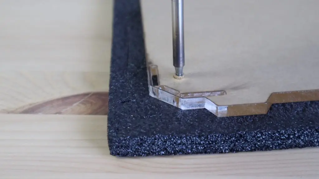
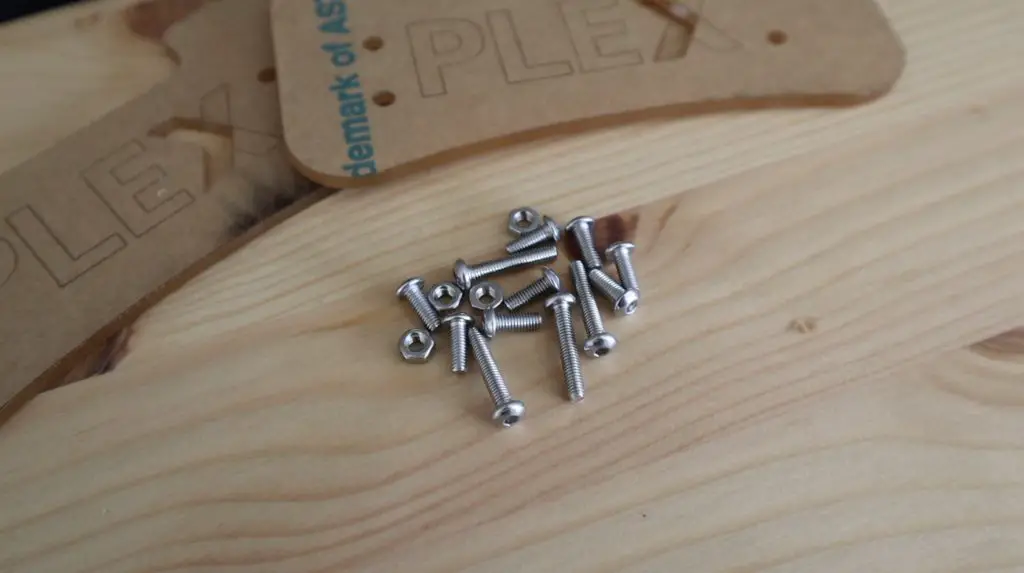
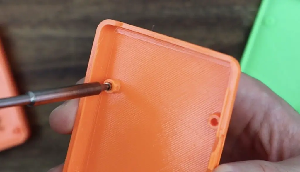
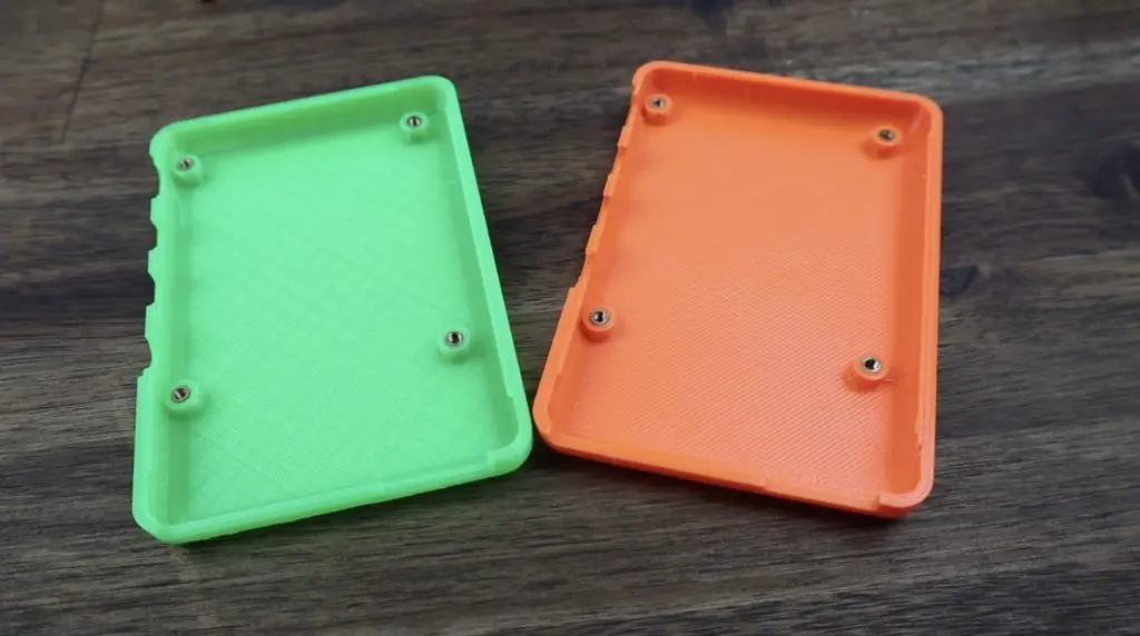
The Pi is held in place with some M2.5 brass standoffs that are secured through the base of the housing with a nut each on the bottom.
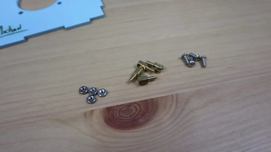
The Pi is then secured to them with an M2.5 screw into each. You can use additional brass standoffs if you want to mount a hat or shield onto your Pi as well.

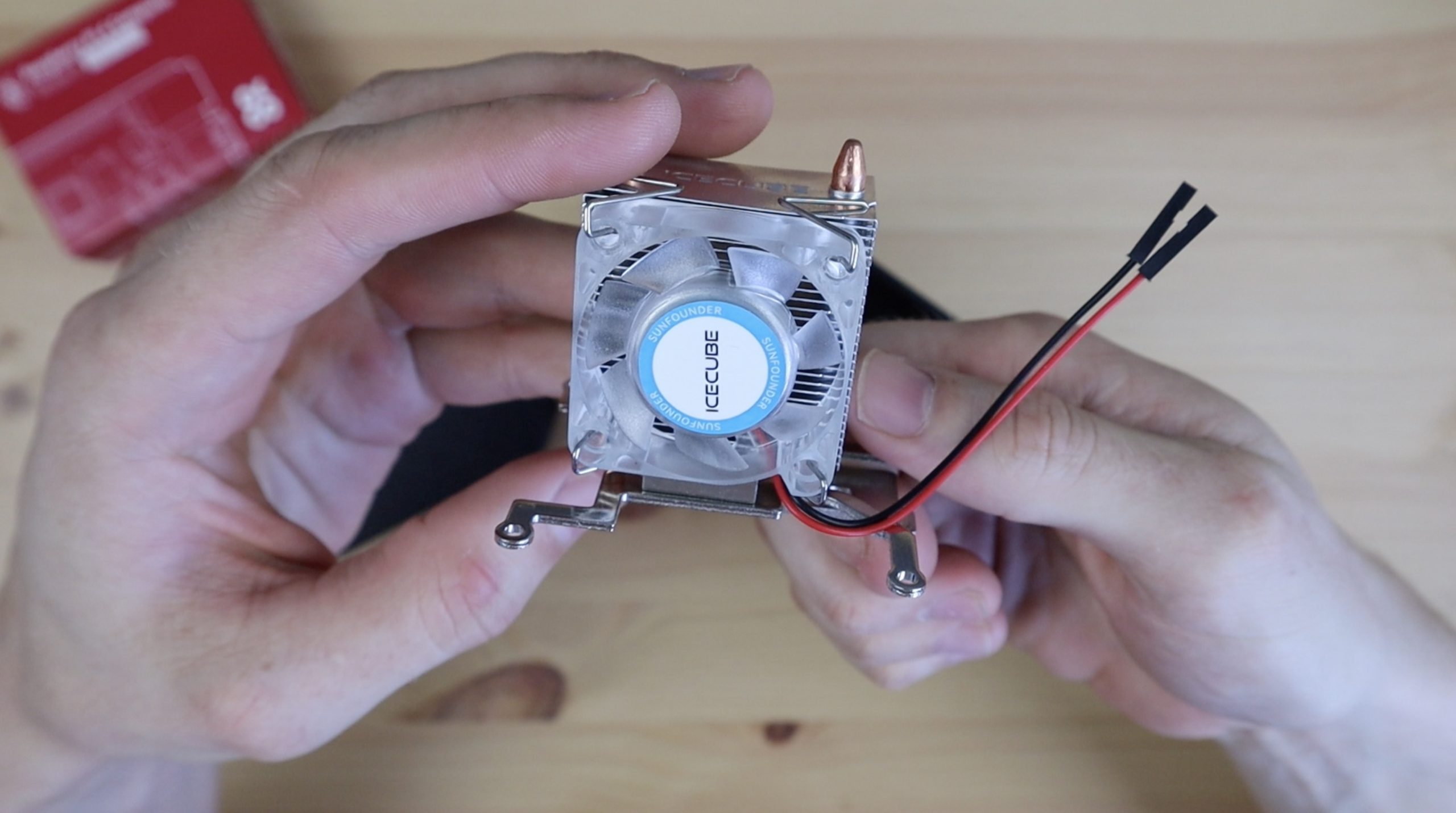
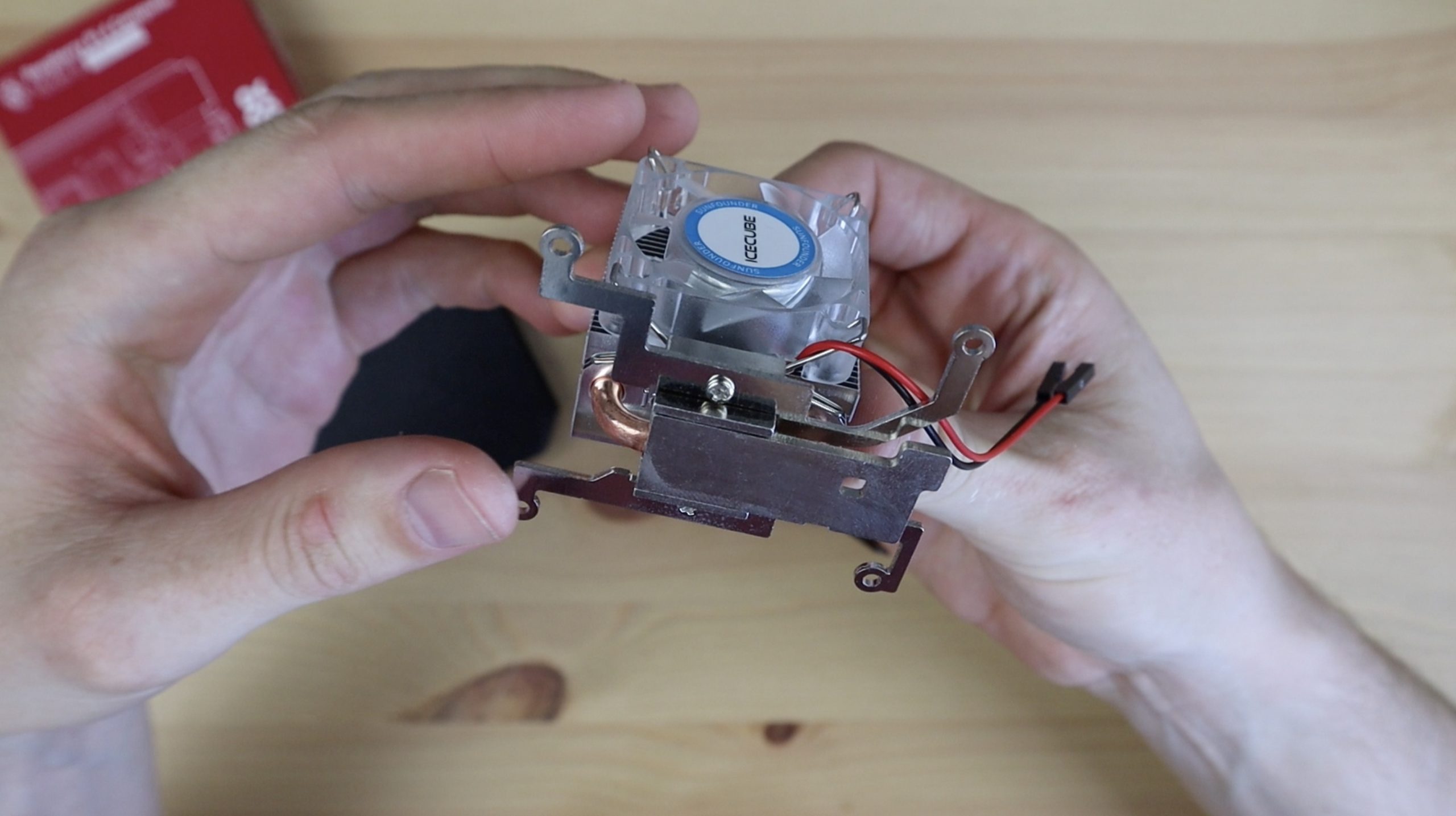
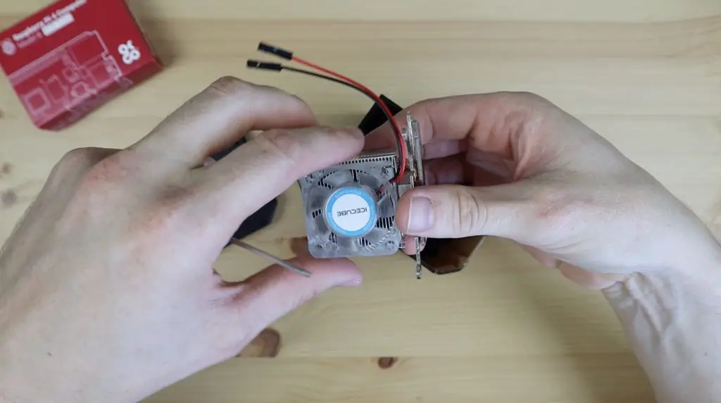
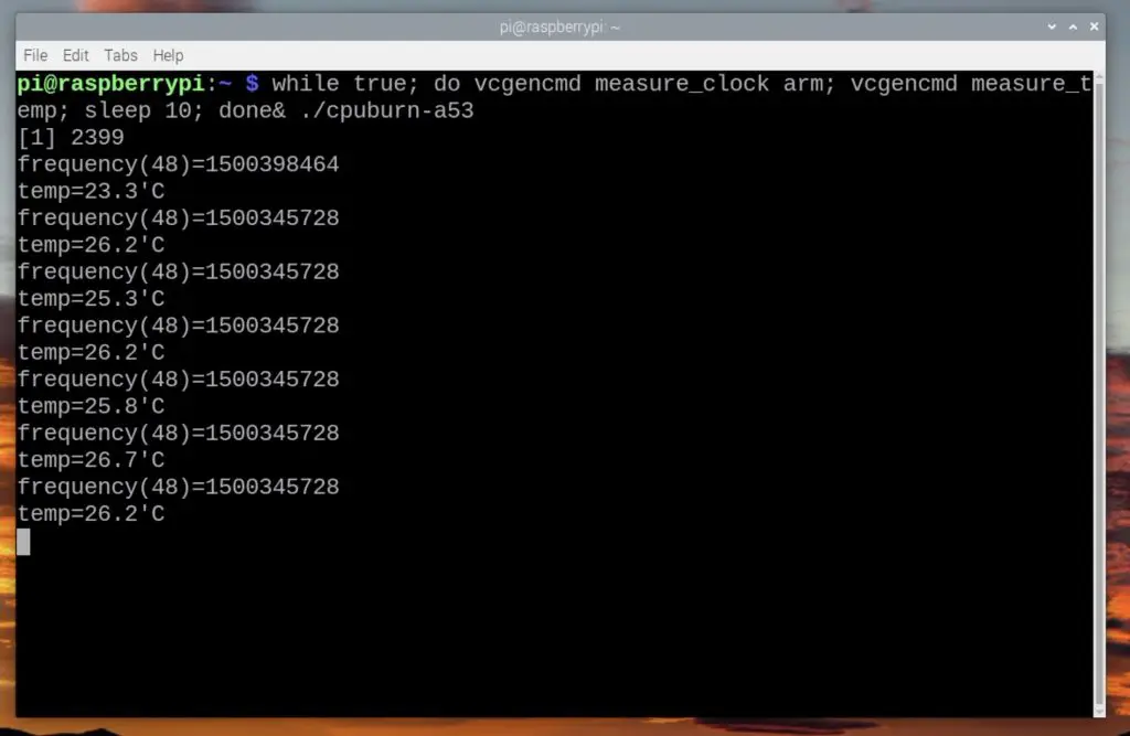
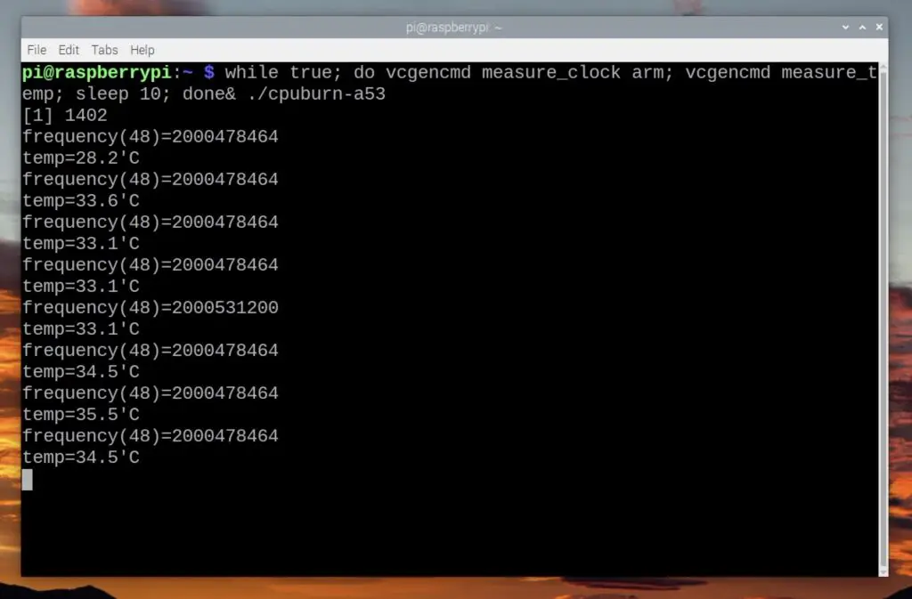
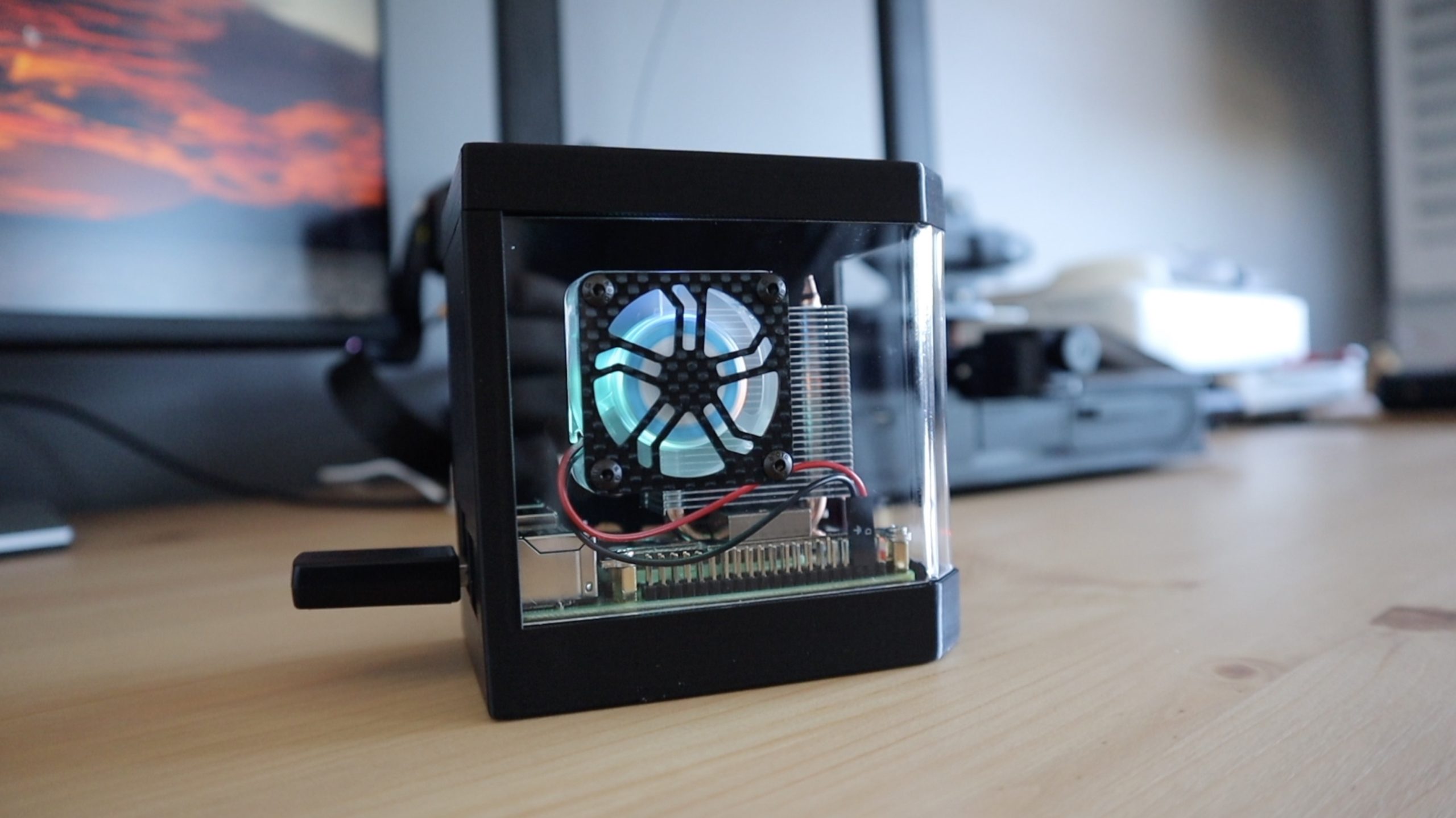
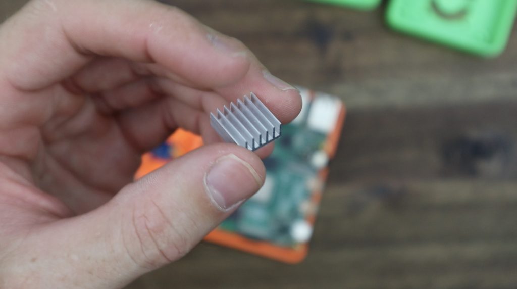
A small aluminium heatsink on the Pi will provide adequate cooling as the CPU isn’t going to be under much load during normal operation.
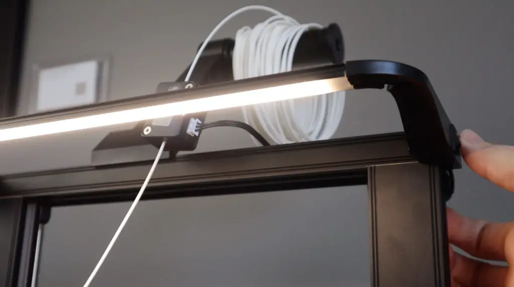
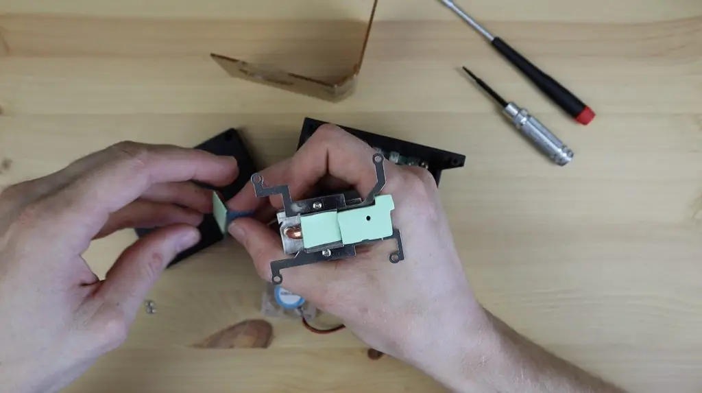
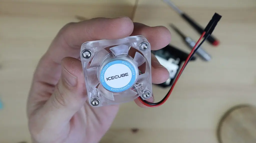
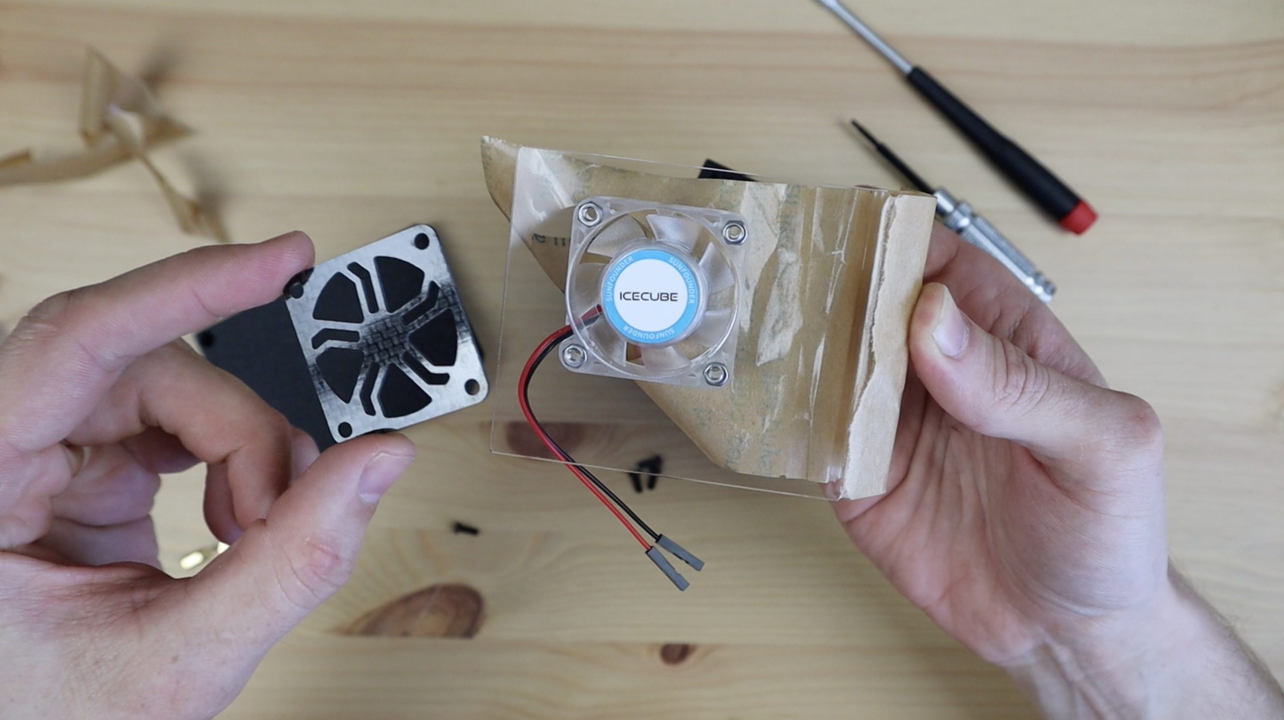
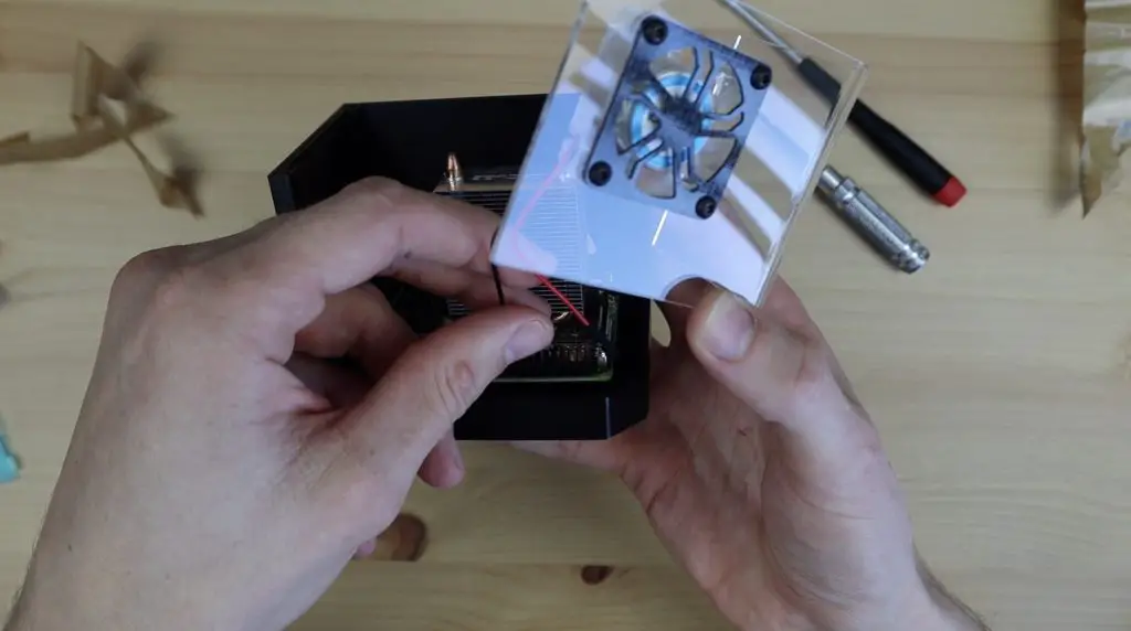
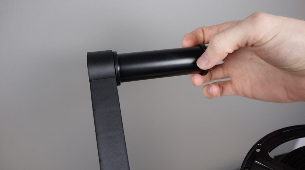
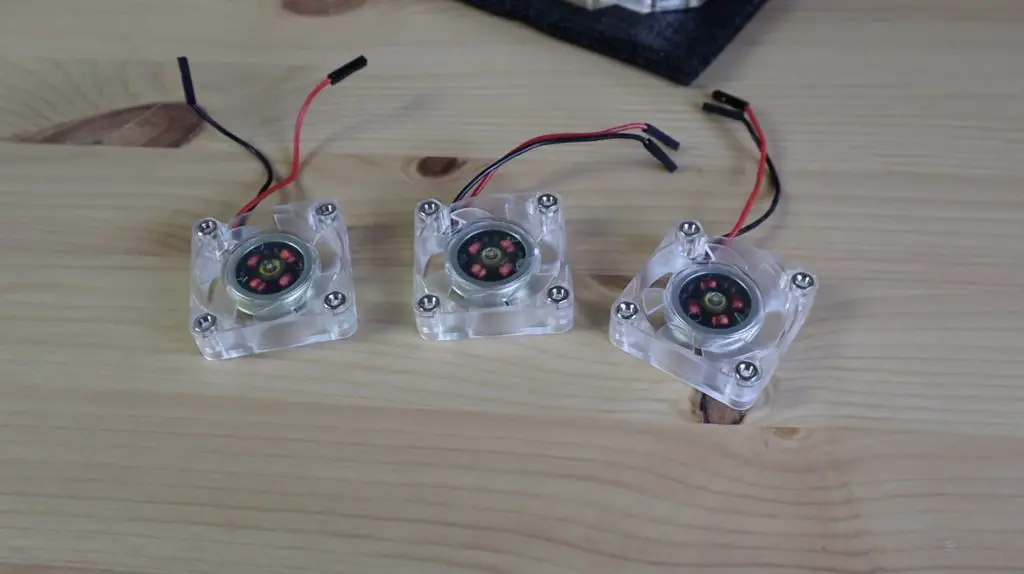
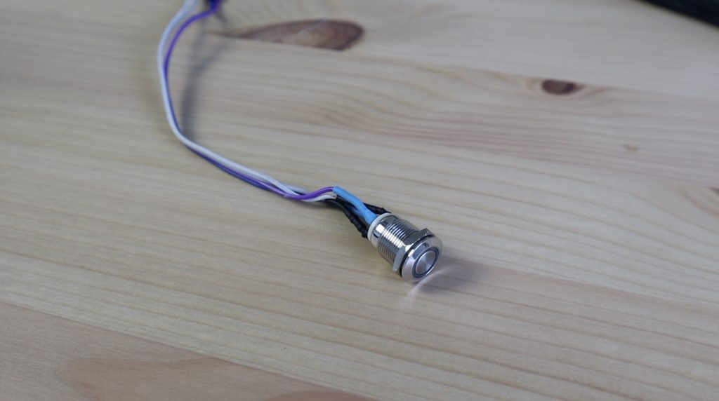
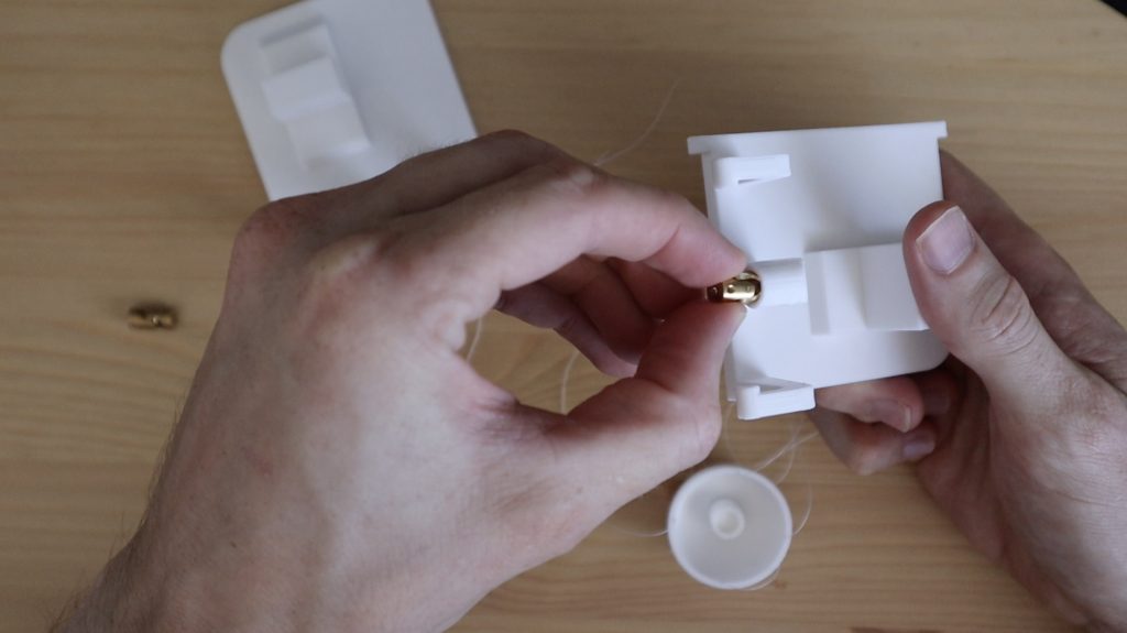
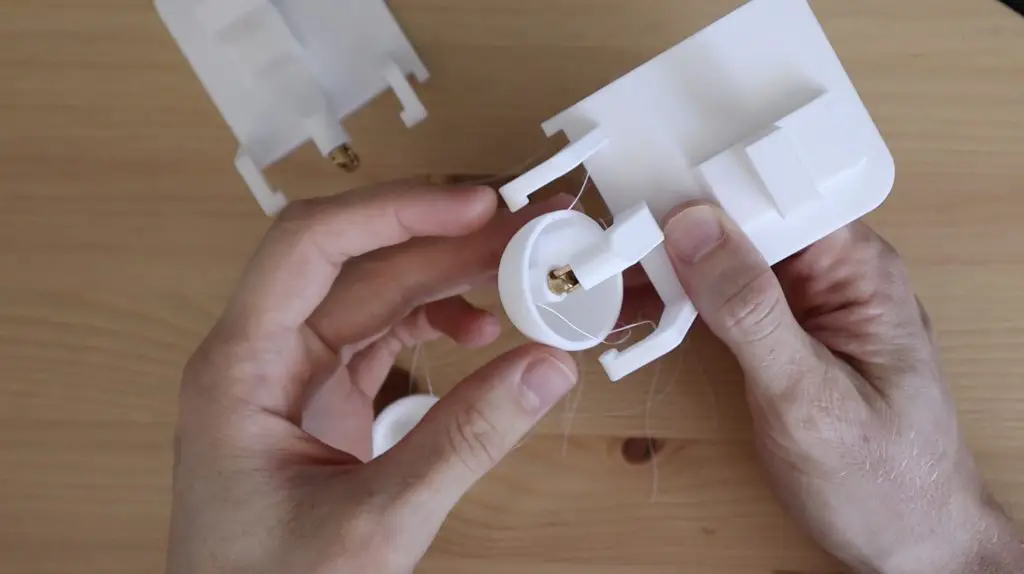
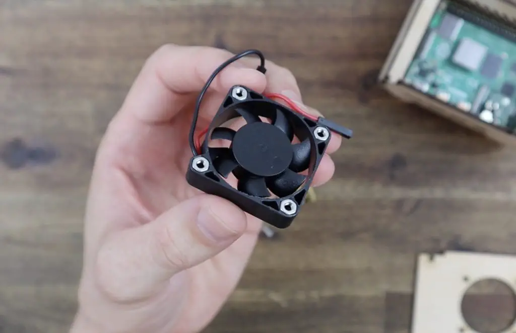
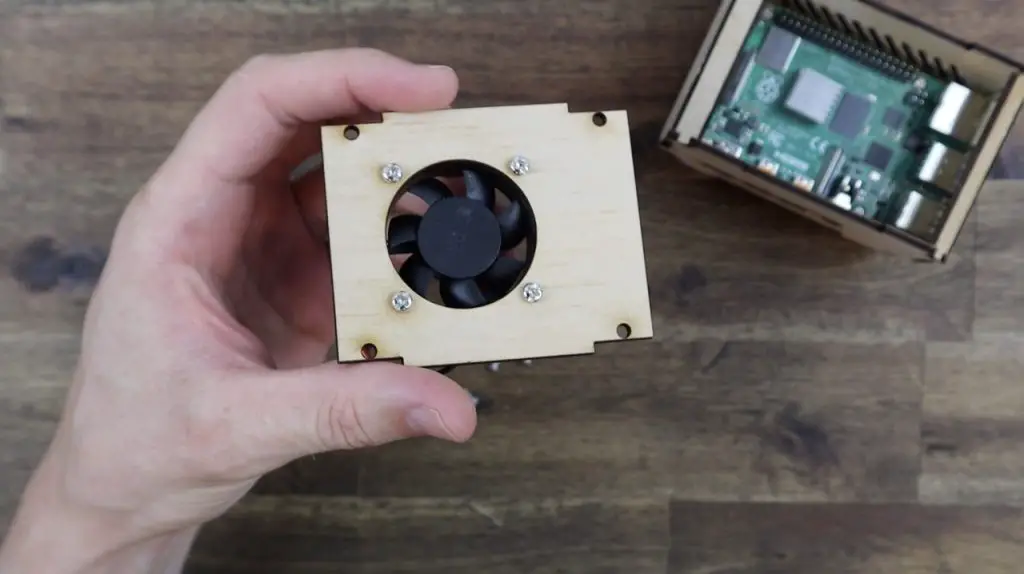
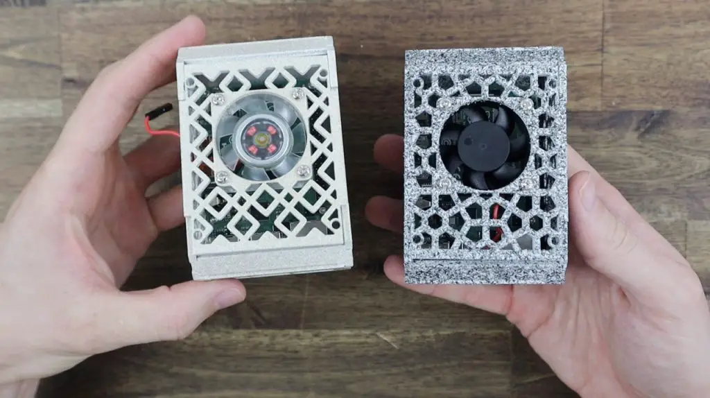
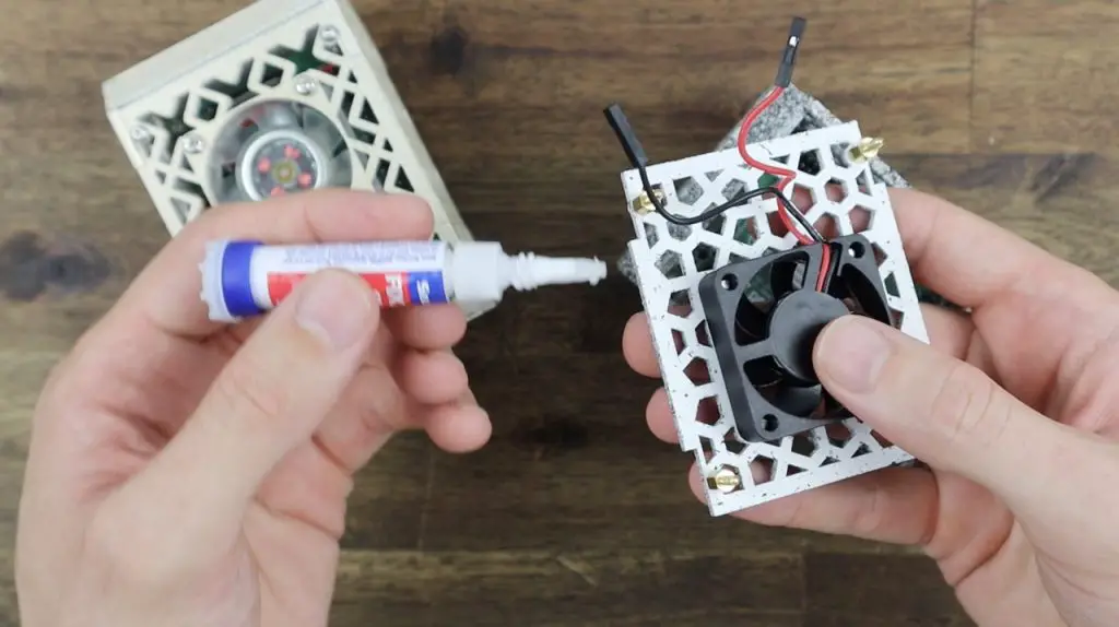
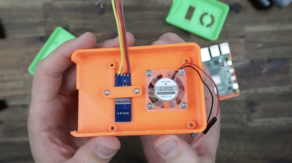
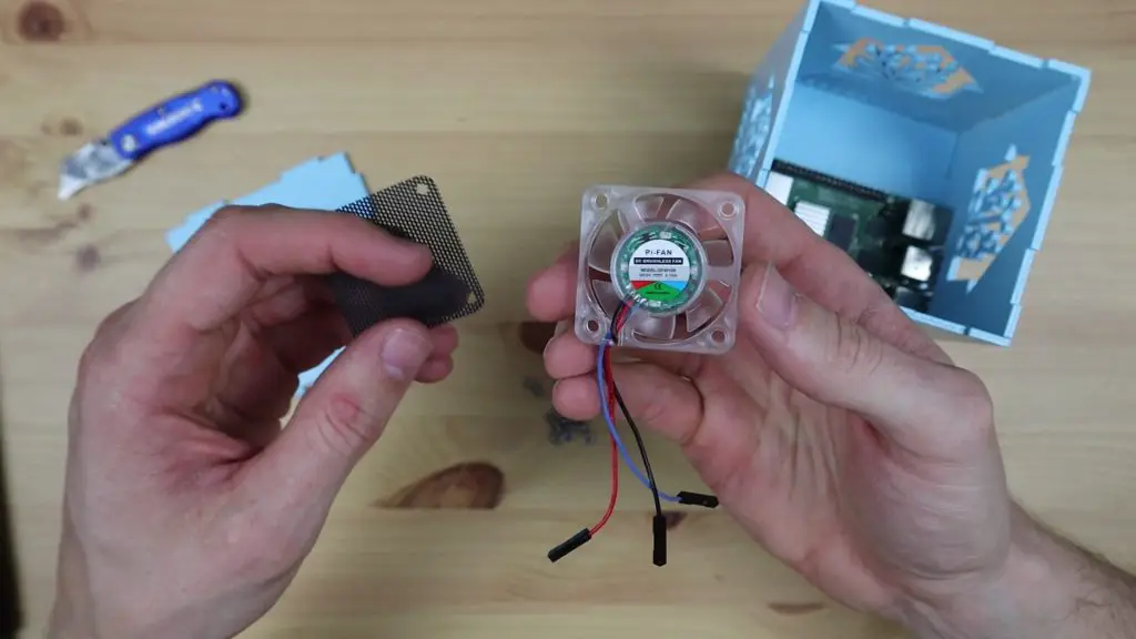
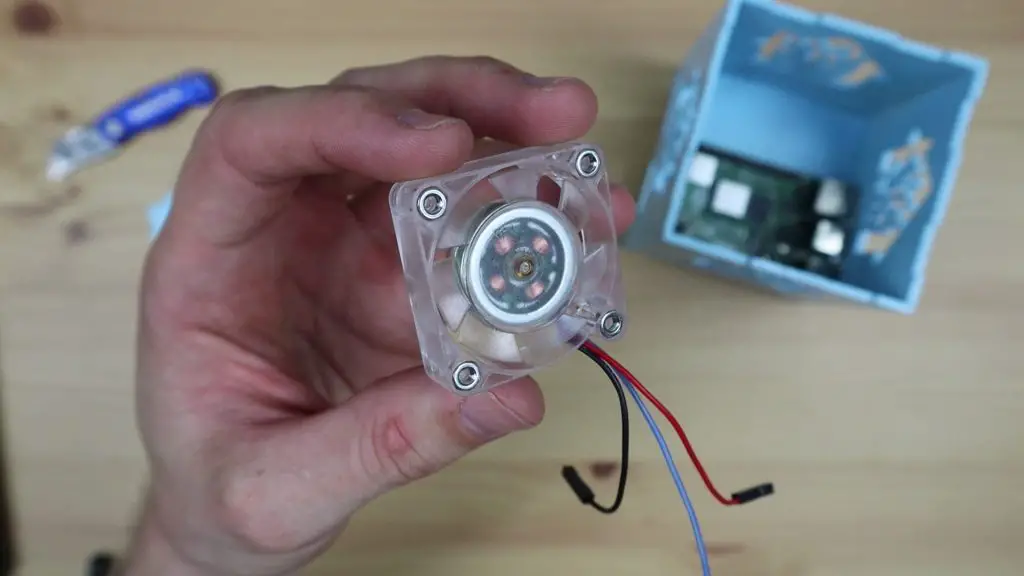
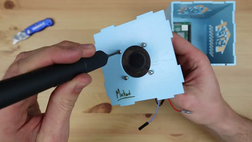
For the fan, I’m going to use a 40mm RGB fan to light up the inside of the case and I’m also going to use a small black dust screen between it and the plywood.
Like I’ve done previously, I’m going to press an M3 nut into each pocket in the fan to screw into. This is easiest done by putting the nuts on a desk or flat surface and pressing the fan pocket down onto them one by one.
The fan and dust screen are then held on the lid with four M3x8mm screws.
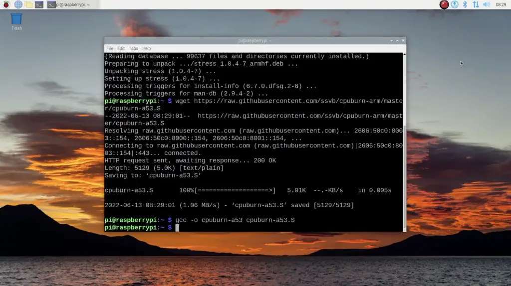
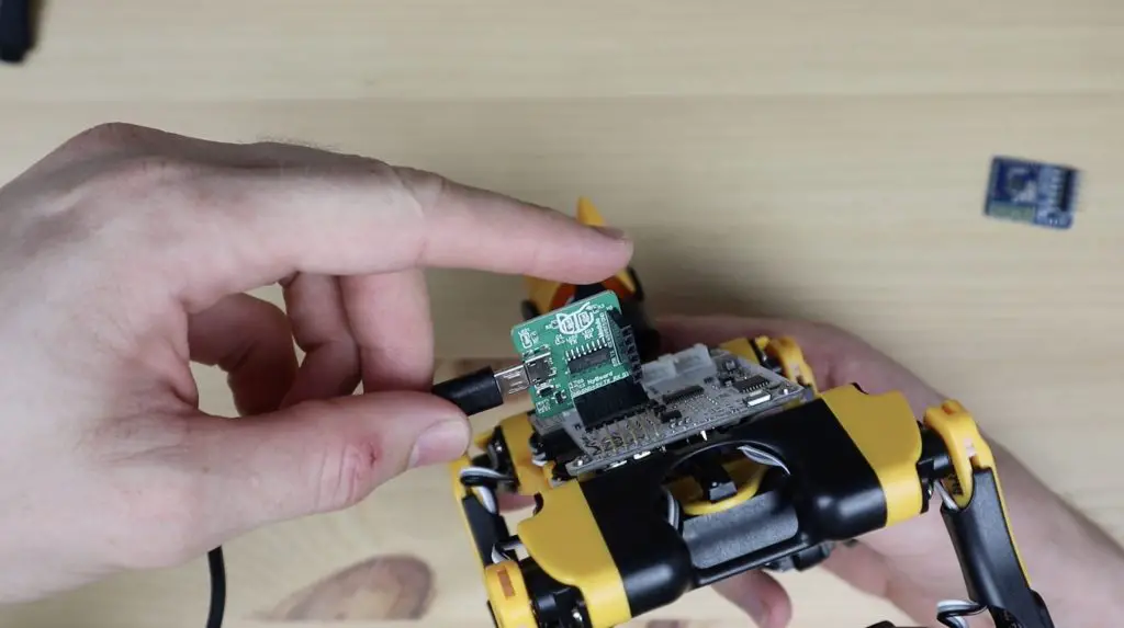
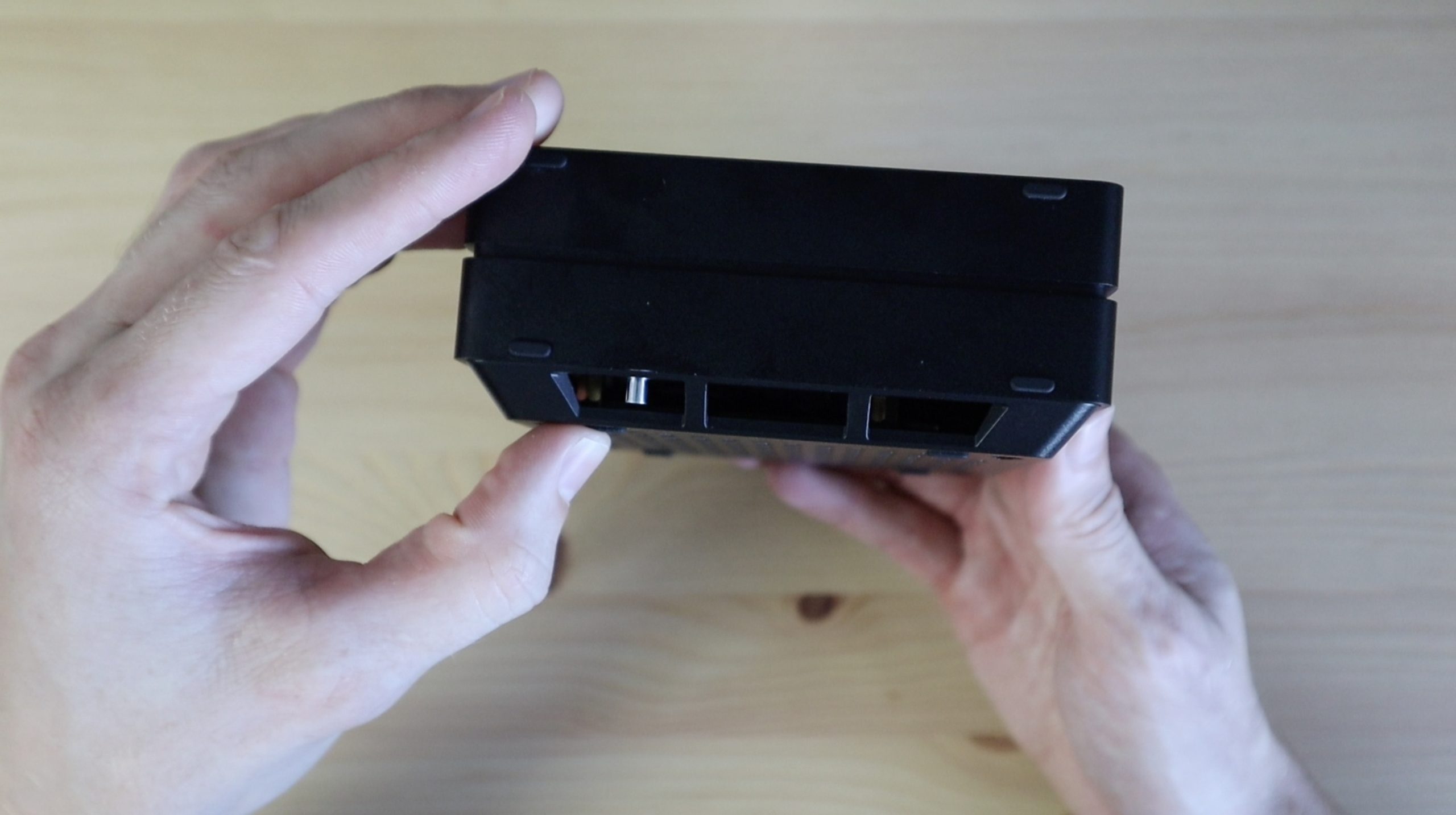
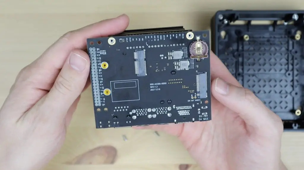
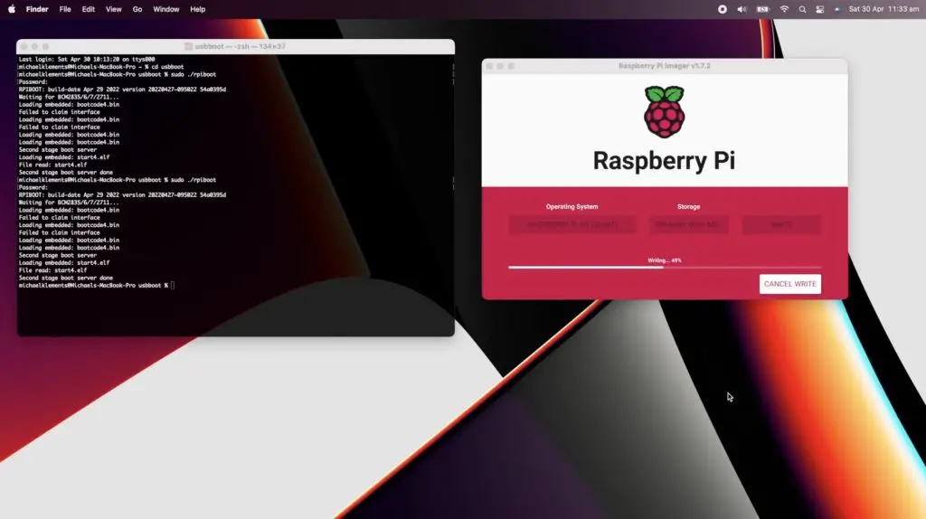
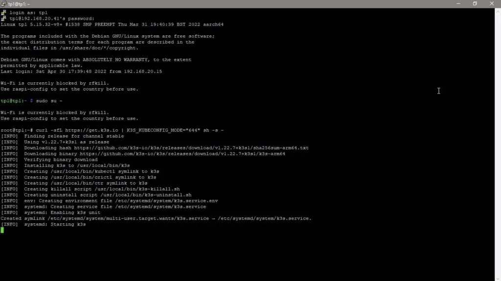
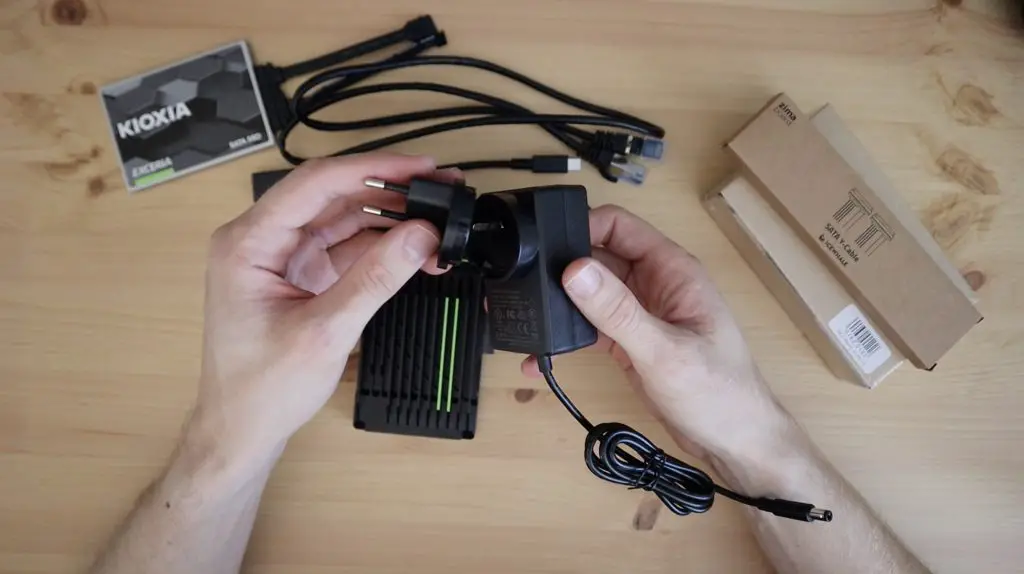
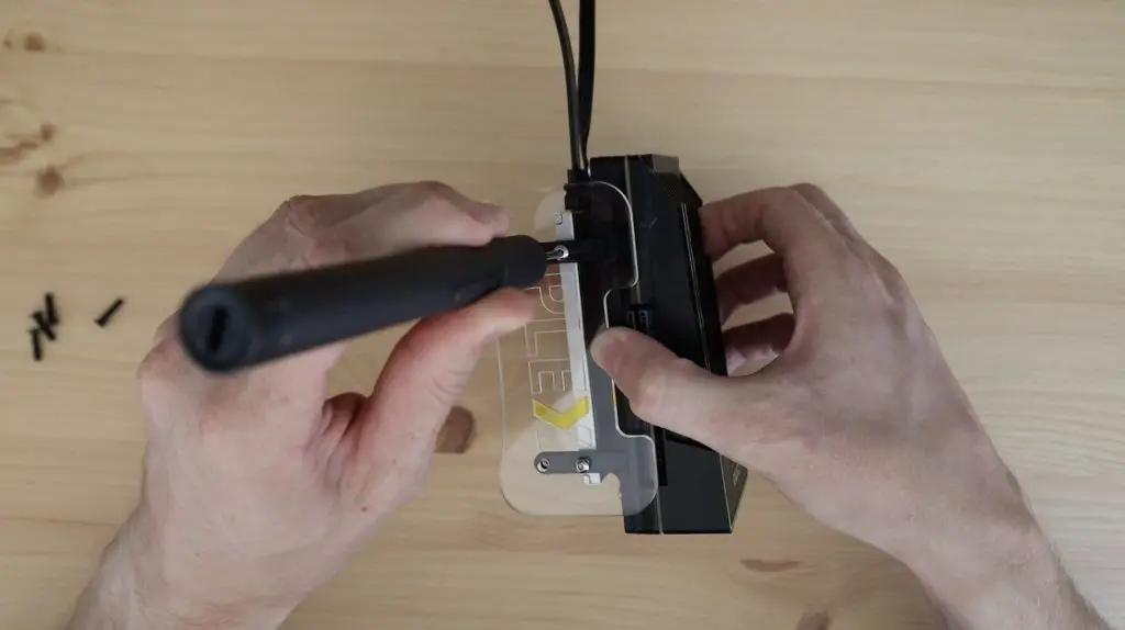
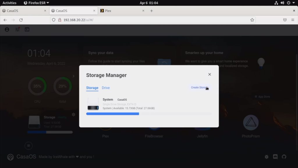
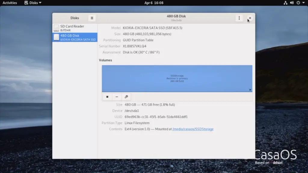
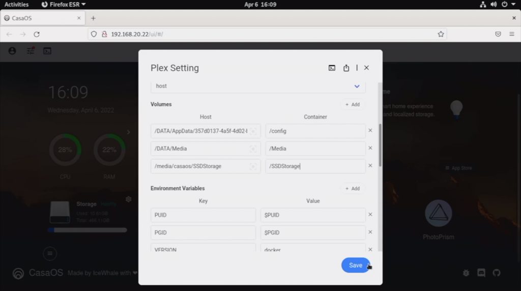
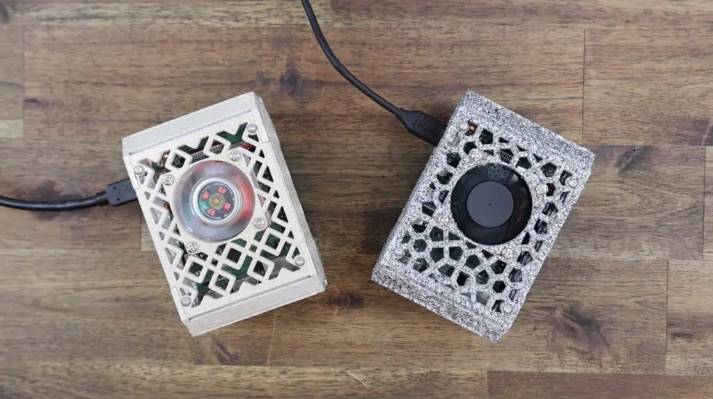
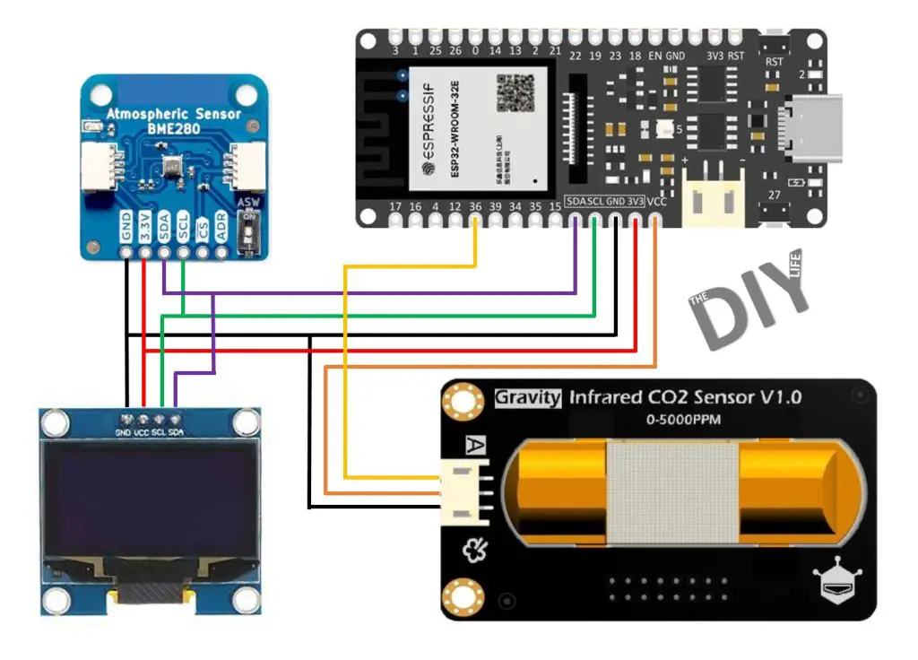
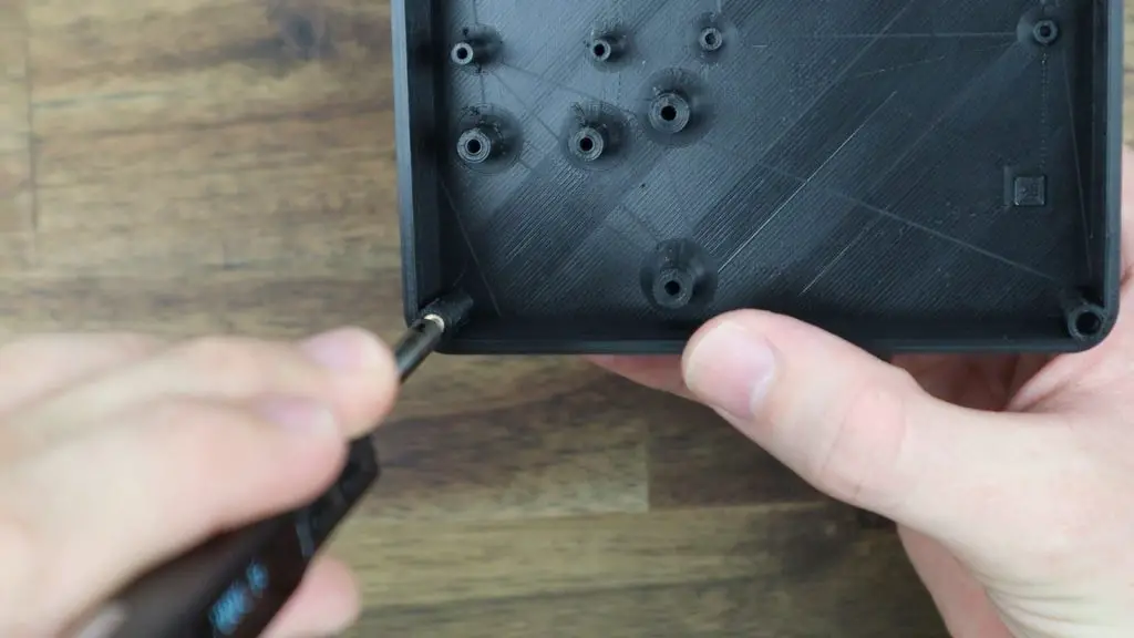
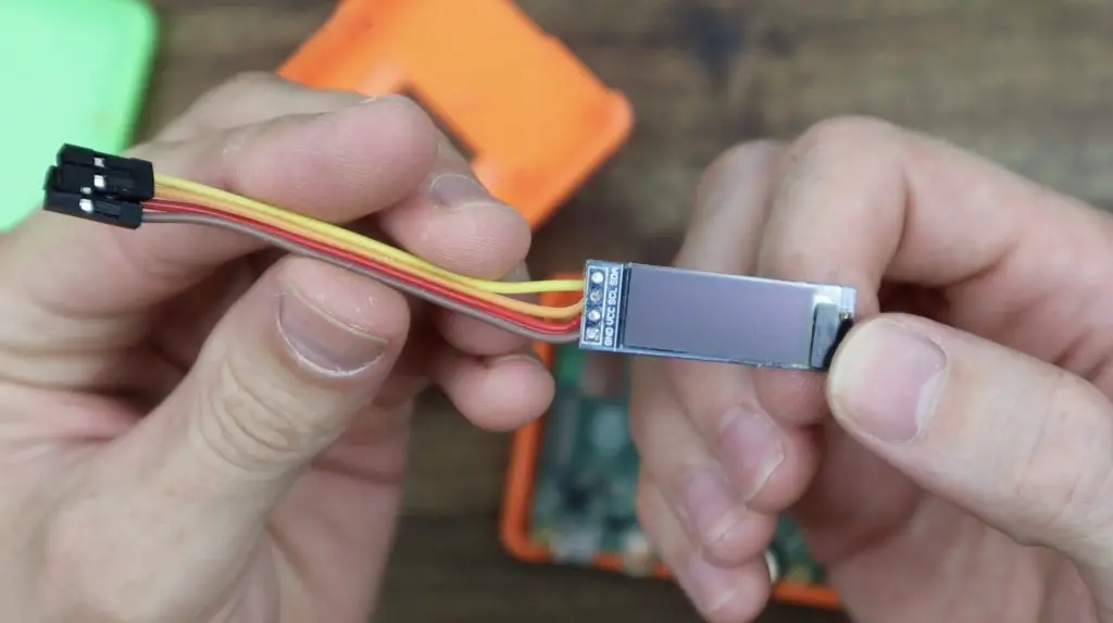
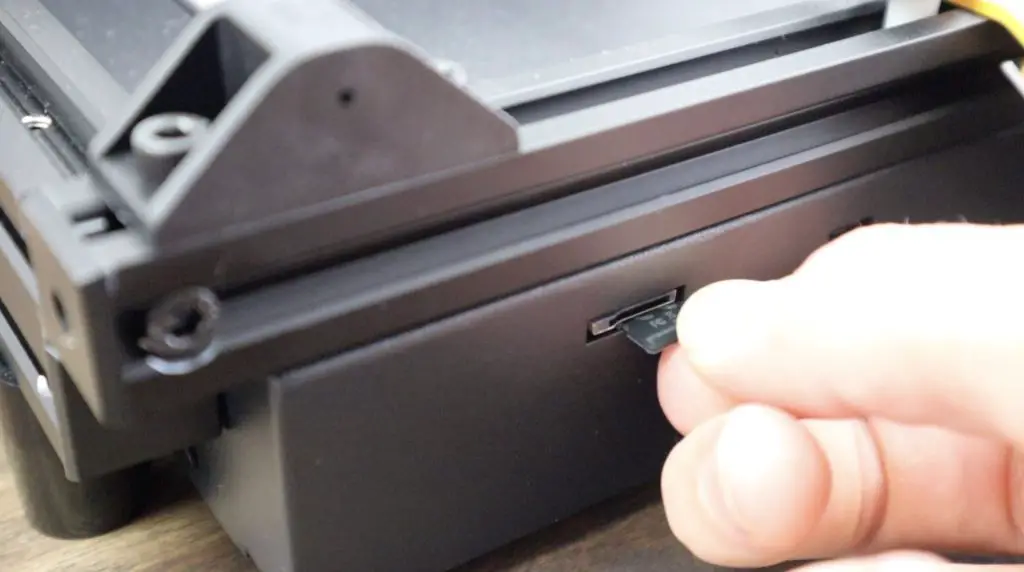
I’m going to flash the home assistant image onto a 32GB Sandisk Ultra microSD card, which we can plug in through the slot on the back of the housing. You’ll probably need to use some tweezers or needle-nose pliers to reach the card slot.
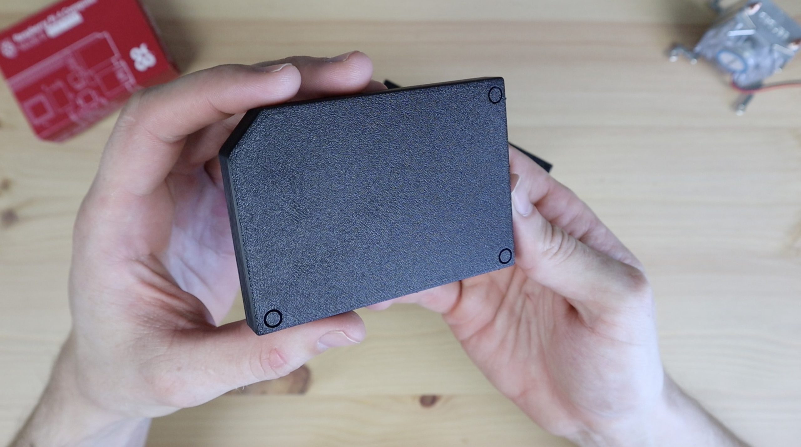
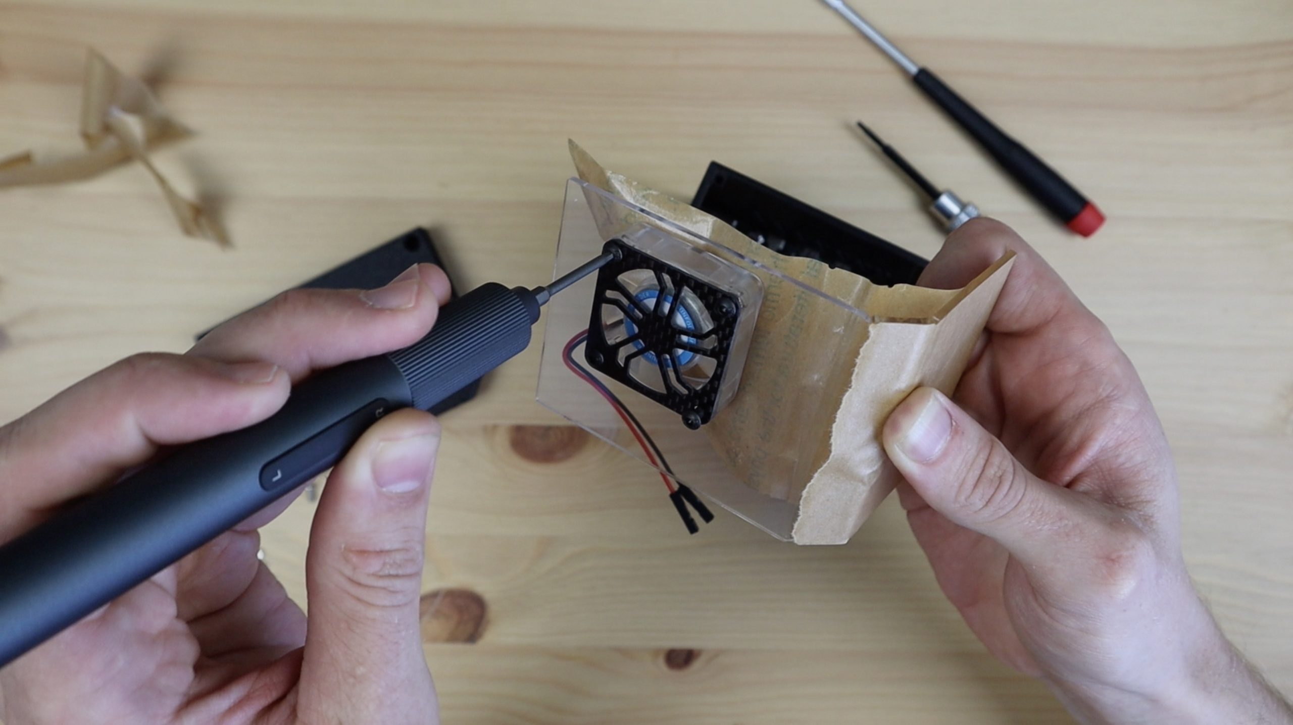
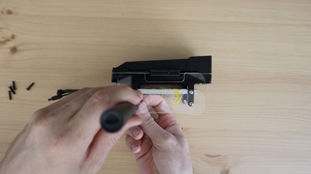
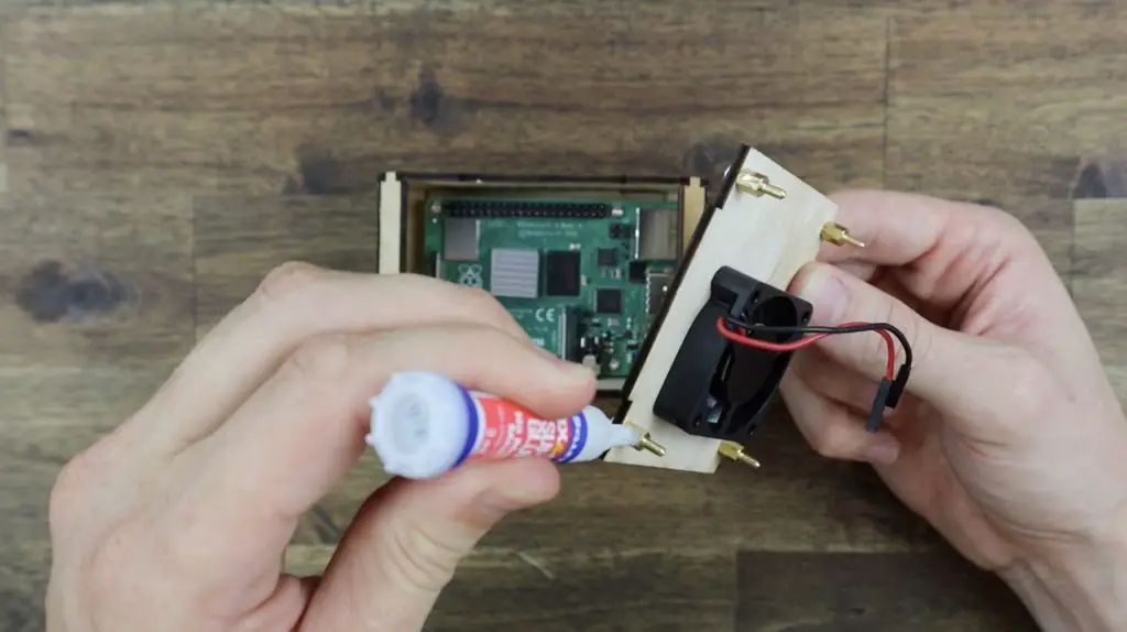
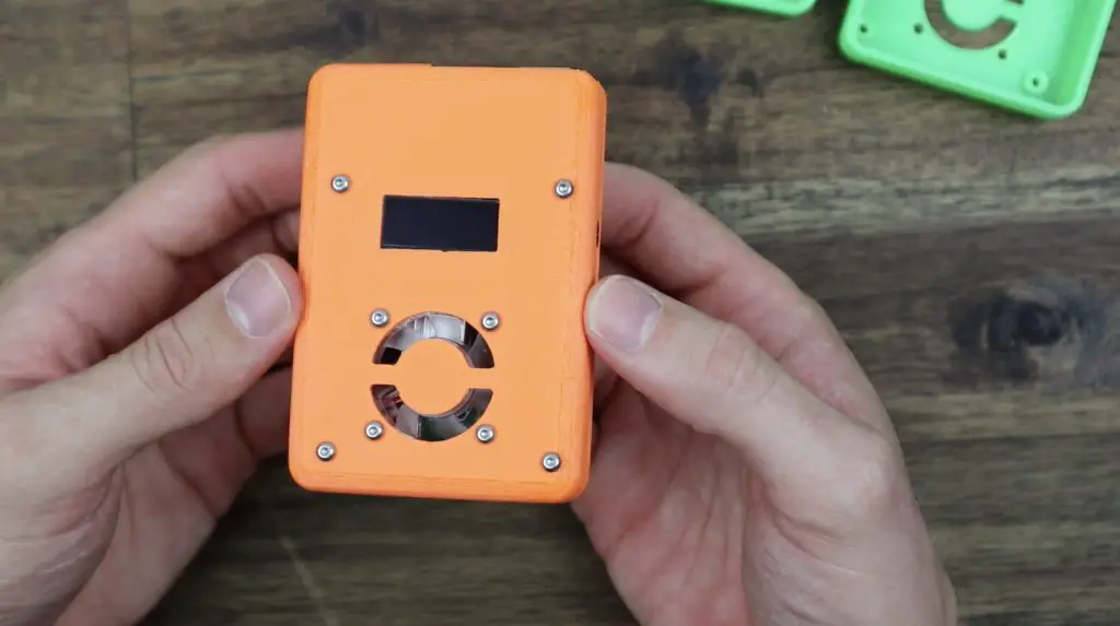
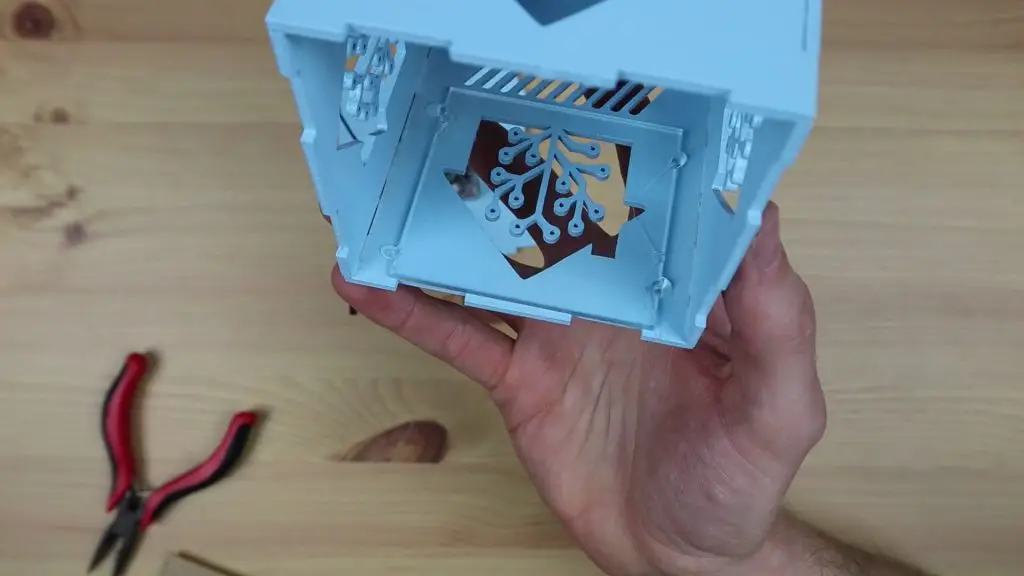
To finish the housing off, I’m going to stick some clear acrylic panels onto the inside behind each logo so that dust cant get in around the logo cutouts. These will also provide a bit of support to the thin branches on the logos so that they’re less likely to get damaged or break off.
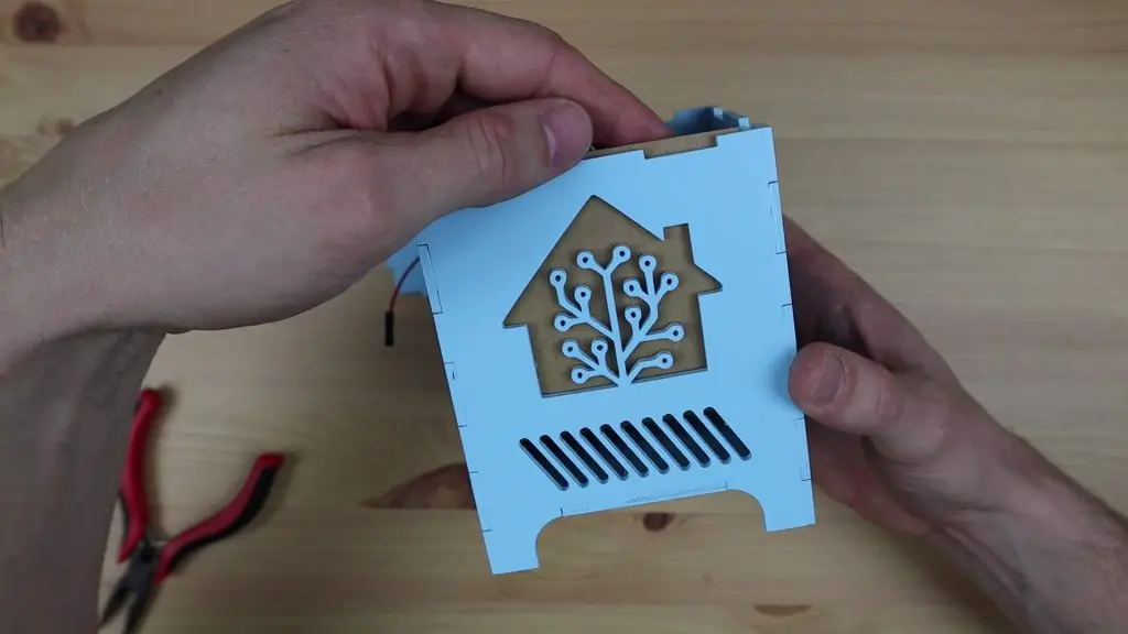
If you don’t have acrylic you can also use some clear plastic sheets or even old containers with clear flat sides.
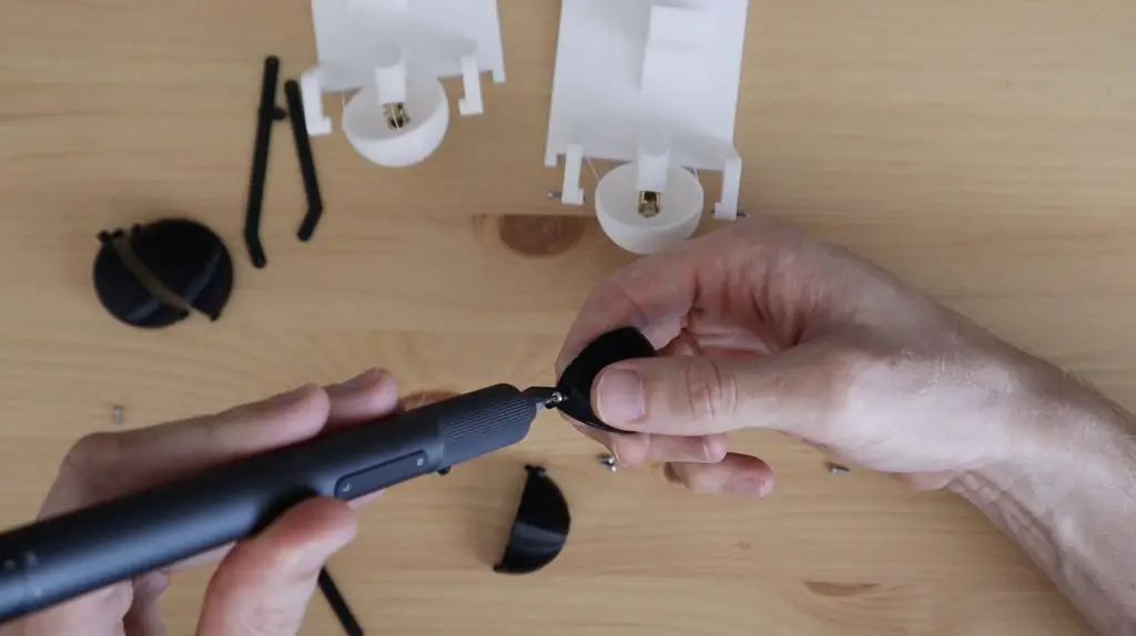
I’m gluing the acrylic in place with hot melt glue in four spots along the edges.
Now we just need to plug the fan into the 5V and GND GPIO pins and we can close up the housing. You can also plug the fan into one of the 3.3V pins if you’d like it to run at a reduced speed and be a bit quiter.
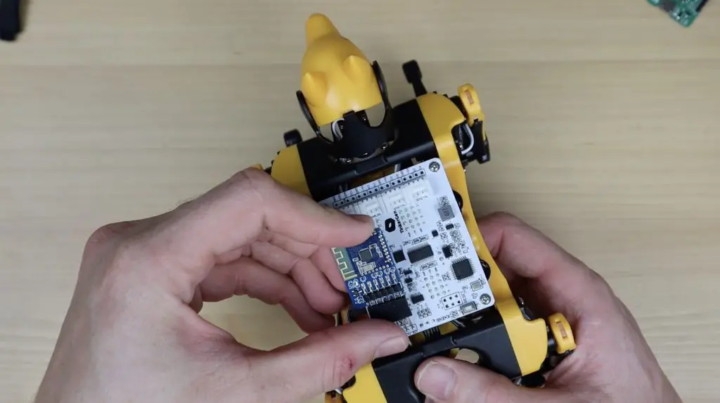
Adding a Zigbee Gateway to the Hub
There are two main low-power communication protocols used by smart home devices – Zigbee and Zwave.

They’re both mesh networks, meaning that every device on the network connects to every other device in range of it and they then dynamically co-operate with each other to send data between nodes through the most efficient route.

I don’t really have a preference between the two, but most of the devices I’ve got so far operate on the Zigbee standard. So, rather than have my Home Assistant hub have to talk to the hub from each manufacturer in order to communicate with its devices and sensors.

I’m going to add a Zigbee gateway to the Home Assistant hub so that it can communicate with them directly.
This will also allow me to use 3rd party Zigbee devices and sensors that don’t have hubs or aren’t part of other ecosystems – so they’re generally cheaper.
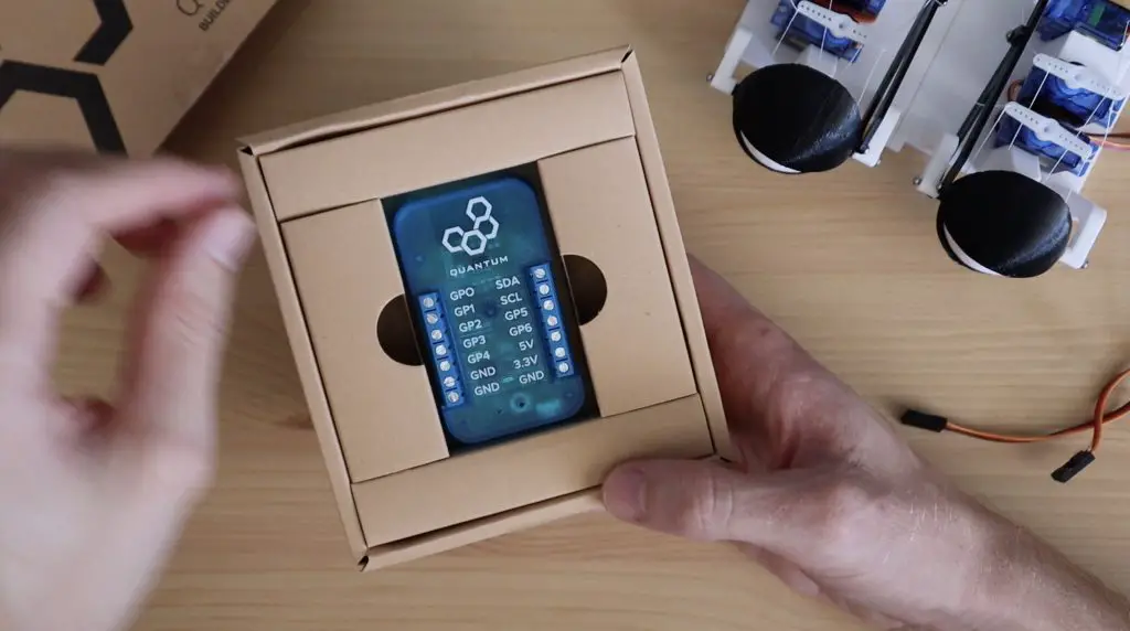
The Gateway I’m going to be using is this little USB adaptor called the ConBee II as it seems to be the most well supported by Home Assistant.
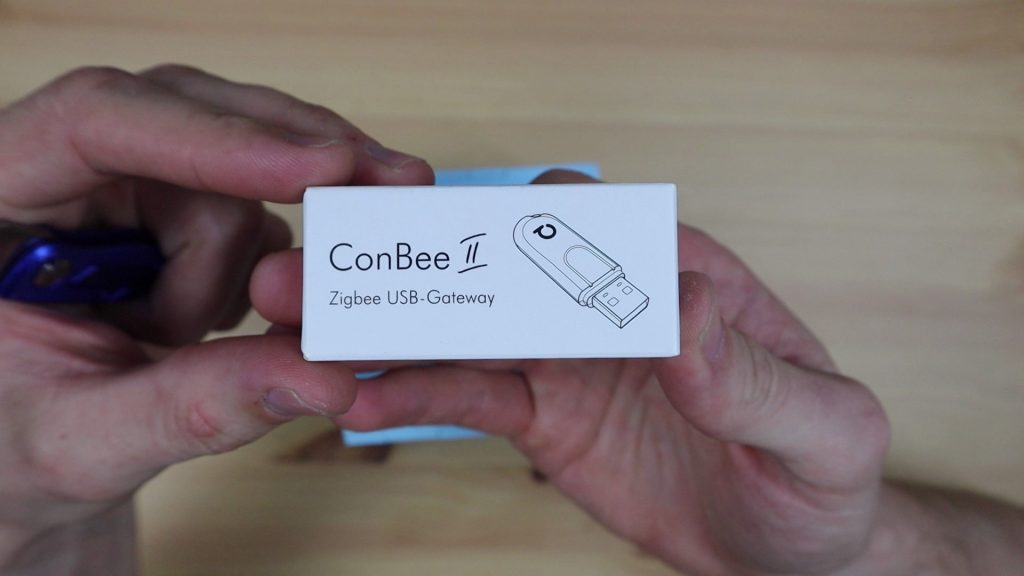
Ideally I’d like to use one that uses the GPIO pins on my Pi so that I can keep it within the housing, so if you know of any that use the Pi’s GPIO pins and work well with Home Assistant please let me know in the comments section at the end of the post.
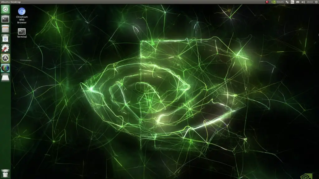
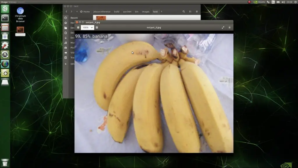
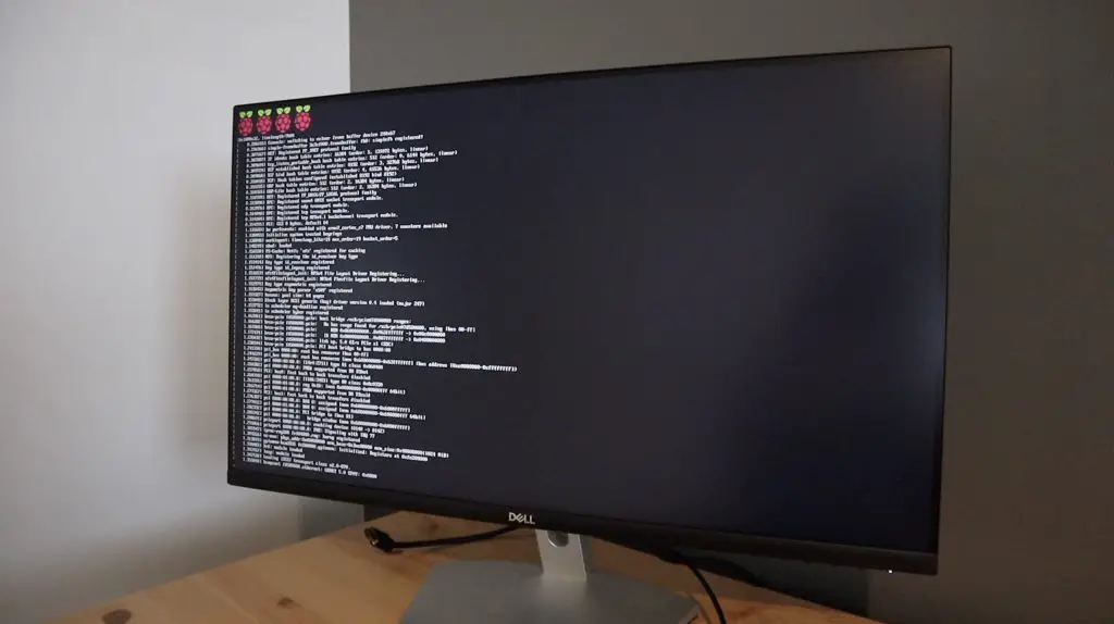
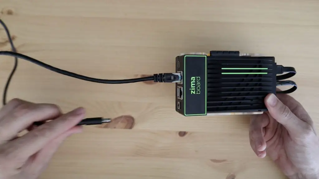
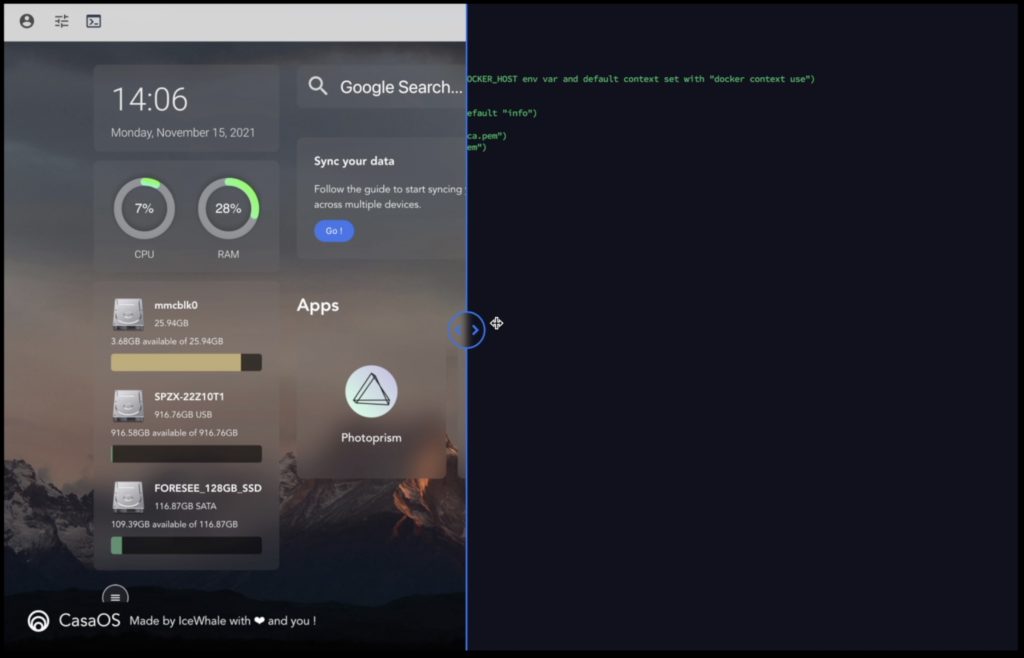
That’s basically it, we’re now ready to start using our new Home Assistant hub to control our smart home devices, let’s get it booted up.
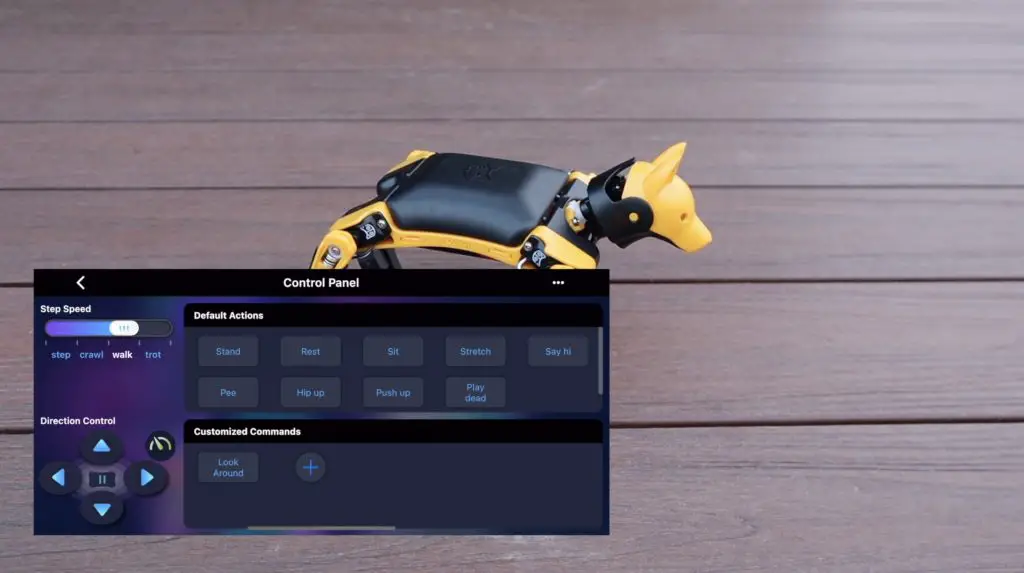
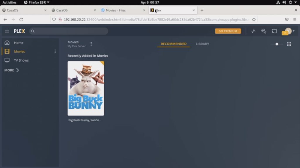
Using the Home Assistant Smart Home Hub
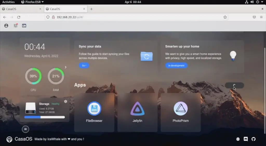
Once set up, you can scan your network to find all of your compatible smart home devices and then start building dashboards, automations and routine to control them.
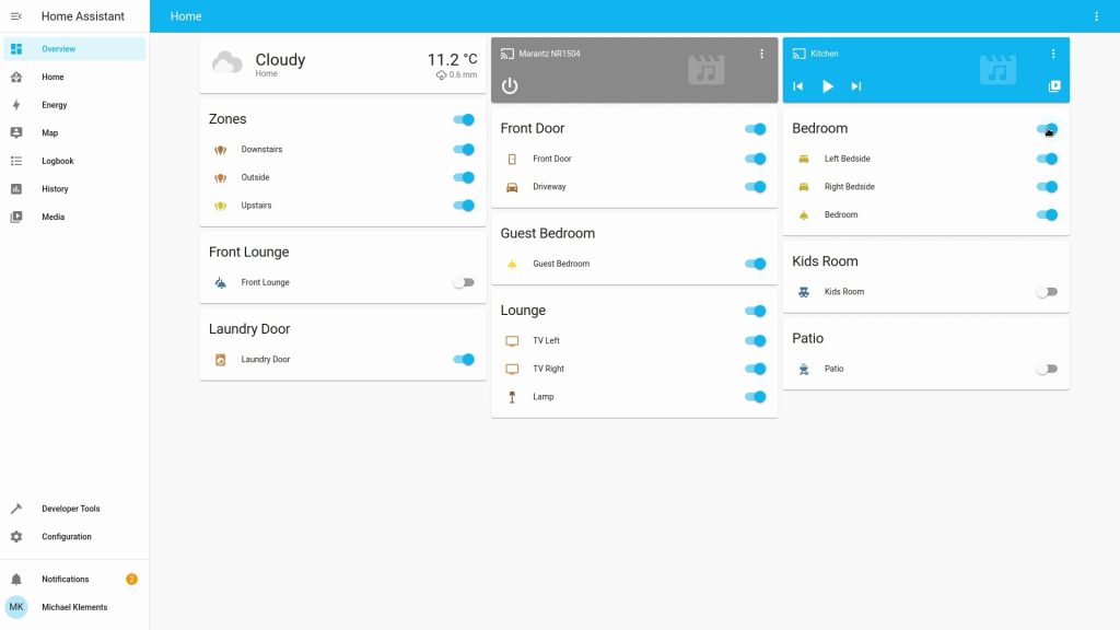
You can access your dashboards through any web browser on your network so you can take control of your home through your laptop, tablet and mobile phone, or even build your own dedicated dashboards with another Raspberry Pi and a touch display.
Check out Smart Home Solver’s channel for some great ideas for home automation routines and automations – he’s got some really creative and unique ideas using a range of sensors and devices.
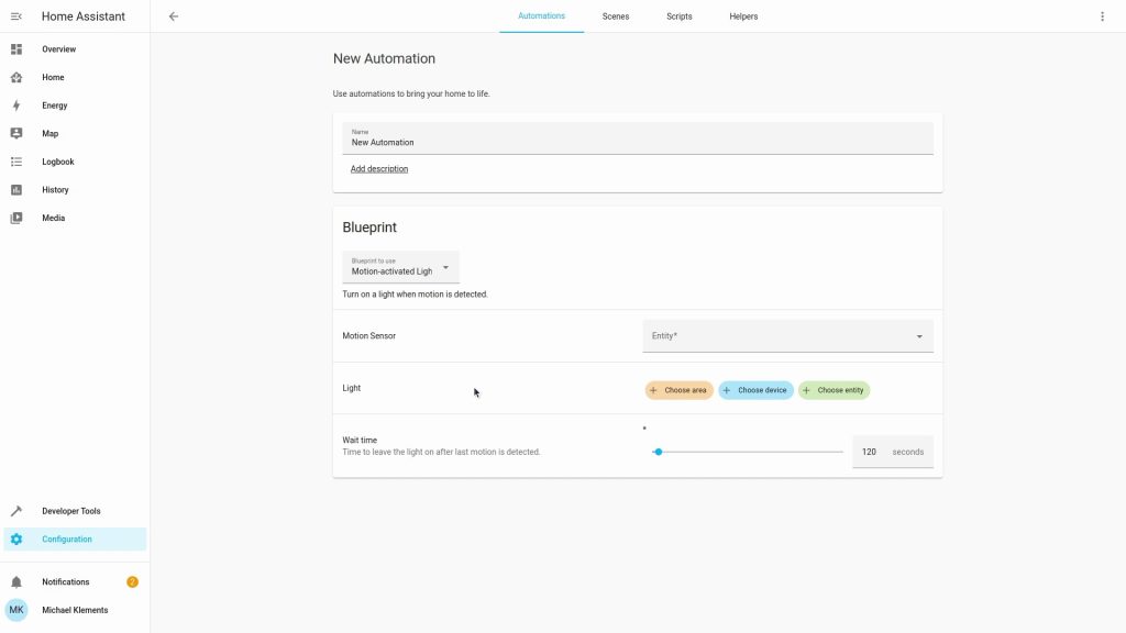
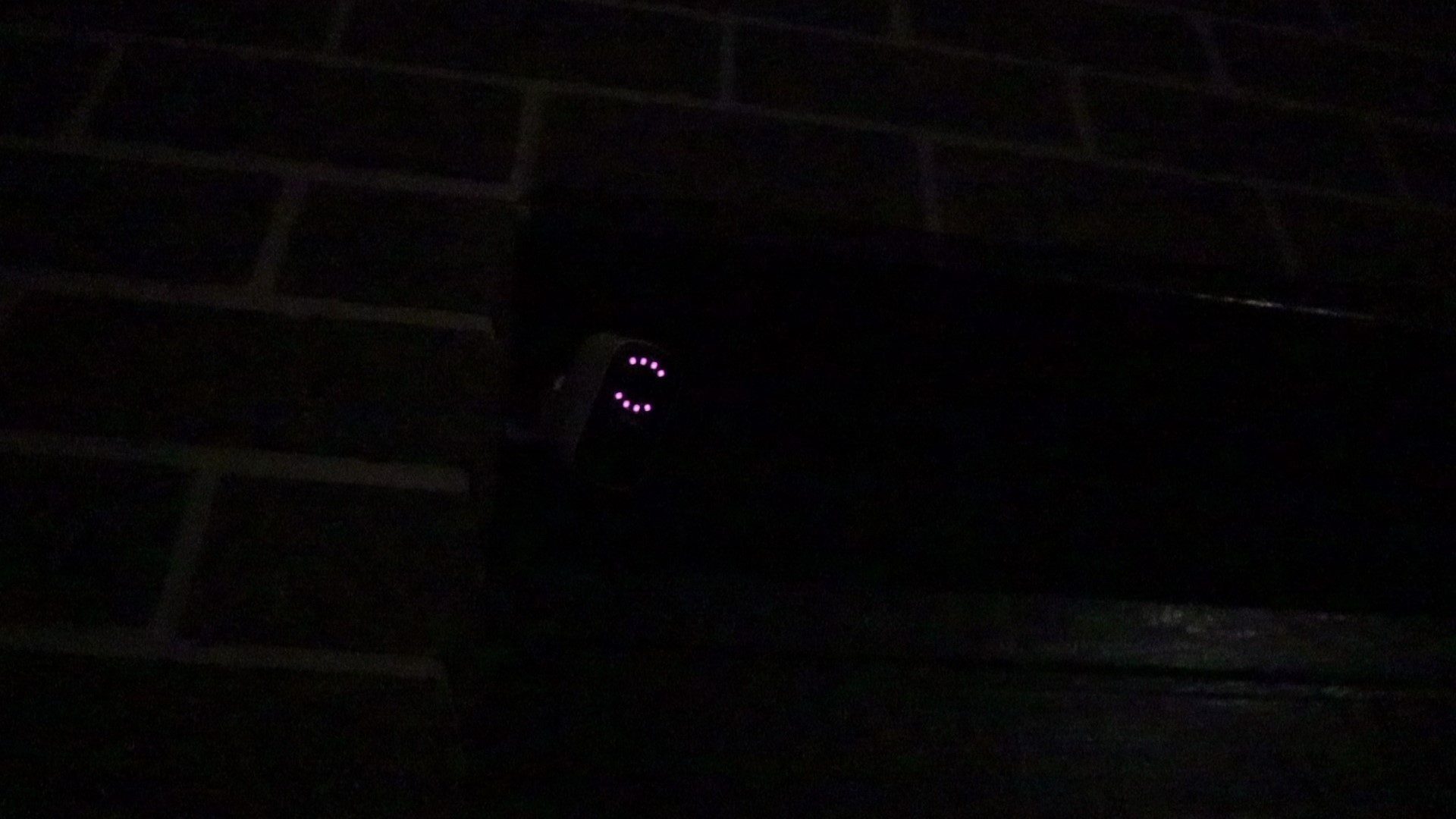
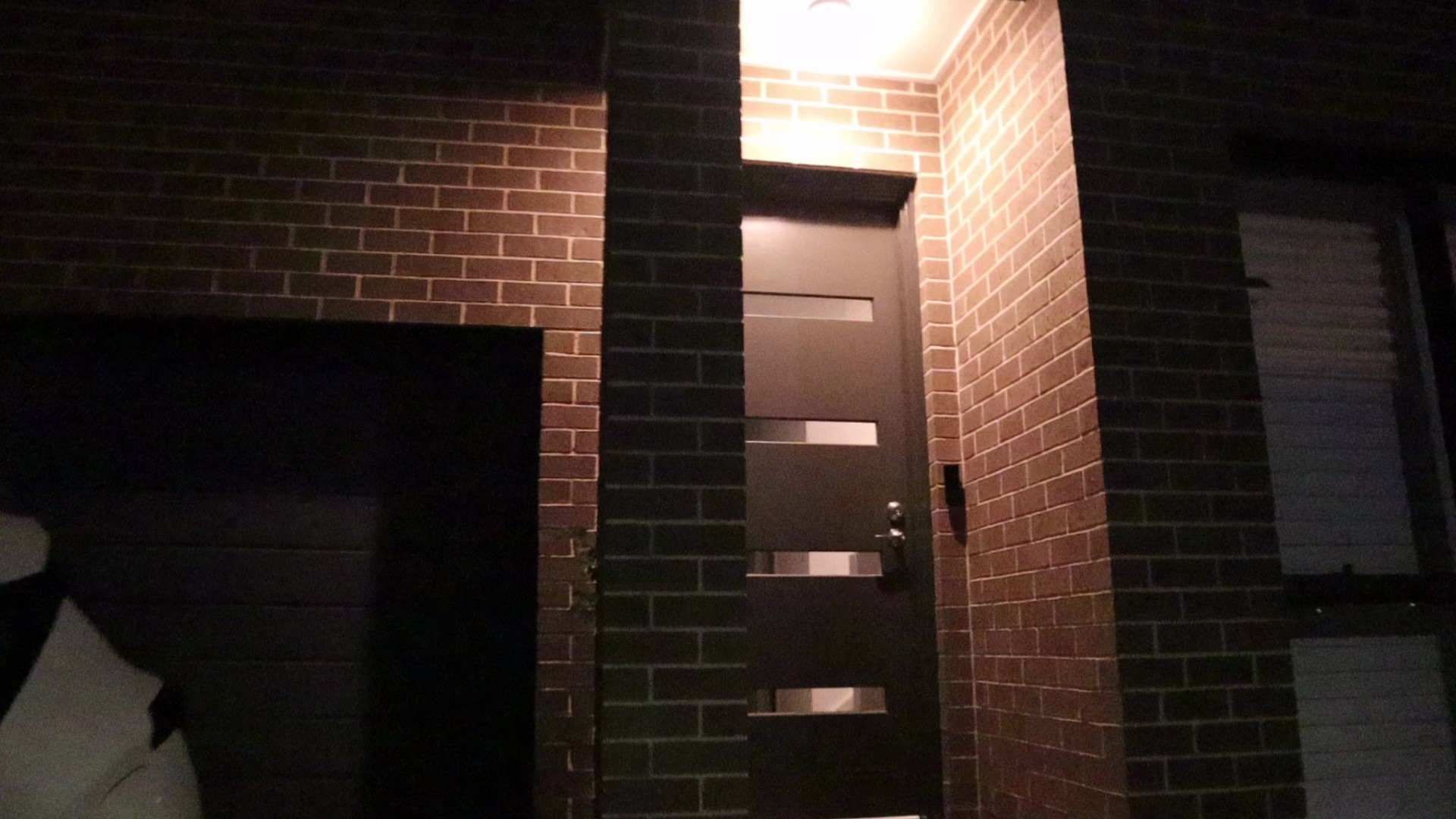
Using Home Assistant I’ve now got the motion sensor on my driveway camera to brighten my porch light for a minute when its on during the evening and it’ll even turn it on for a minute during the night if its off.
Next I’m going to be setting up some motion sensors or magnetic switches to turn on my pantry and closet lights when the doors are open.
Final Thoughts on the Atomstack X20 Pro
The Atomstack X20 Pro is without a doubt the best diode laser machine I’ve personally used. The powerful laser allows you to work with thicker materials and is now actually quite useful for thinner ones as well. I’m able to cut 3mm plywood three to four times faster than I could with a 5W laser. So it’s actually becoming a worthwhile alternative to my CO2 laser at this point.
The air assist works really well to get cleaner cuts and engravings and won’t leave your eardrums ringing after you’ve used it. And finally, the inclusion of WiFi and a phone app means that you’ve got another way to easily use the X20 Pro, streamlining your workflow.
I’ll definitely be looking to add a honeycomb mesh bed to the X20 Pro and I need to design an enclosure for it so that I can contain and direct the smoke out of my workshop.
Let me know what you think of the Atomstack X20 Pro in the comments section below. Also let me know if you’ve used Home Assistant in your home and what interesting devices and automations you’ve set up.